
Histograms, Pie Charts, and Animations
Overview
In this section we’ll explore some more specialized plot types, including:
Histograms
Pie Charts
Animations
Imports
The same as before, we are going to import Matplotlib’s pyplot interface as plt.
import matplotlib.pyplot as plt
import numpy as np
Histograms
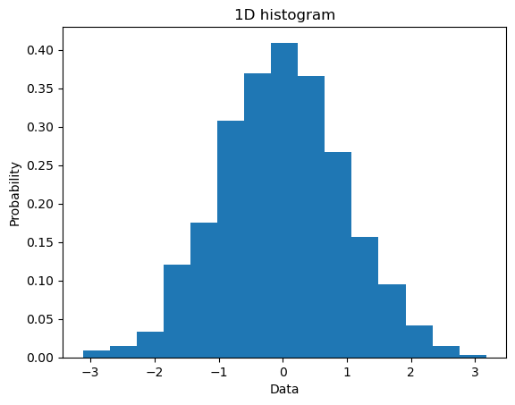
To make a 1D histogram, we’re going to generate a single vector of numbers.
We’ll generate these numbers using NumPy’s normal distribution random number generator. For demonstration purposes, we’ve specified the random seed for reproducability.
npts = 2500
nbins = 15

np.random.seed(0)
x = np.random.normal(size=npts)
Finally, make a histogtam using plt.hist. Here, specifying density=True changes the y-axis to be probability instead of count.
plt.hist(x, bins=nbins, density=True)
plt.title('1D histogram')
plt.xlabel('Data')
plt.ylabel('Probability');
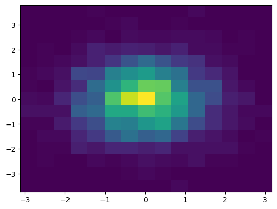
Similarly, we can make a 2D histrogram by generating a second random array and using plt.hist2d.
y = np.random.normal(size=npts)

plt.hist2d(x, y, bins=nbins);
Pie Charts
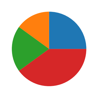
Matplotlib can also be used to plot pie charts with plt.pie. The most basic implementation is shown below. The input to plt.pie is a 1-D array of wedge “sizes” (e.g. percent values).
x = np.array([25, 15, 20, 40])
plt.pie(x);
Typically, you’ll see examples where all of the values in the array x will sum to 100, but the data provided to the pie chart does NOT have to add up to 100. Any numbers provided will be normalized to sum(x)==1 by default, although this can be turned off by setting normalize=False.
If you set normalize=False and the values of x do not sum to 1 AND are less than 1, a partial pie will be plotting. If the values sum to larger than 1, a ValueError will be raised.
x = np.array([0.25, 0.20, 0.40])
plt.pie(x, normalize=False);

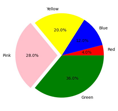
Let’s do a more complicated example.
Here we create a pie chart with various sizes associated with each color. Labels are derived by capitalizing each color in the array colors.
More interesting is the explode input, which allows you to offset each wedge by a fraction of the radius. In this example, each wedge is not offset except for the pink (3rd index).
colors = ['red', 'blue', 'yellow', 'pink', 'green']
labels = [c.capitalize() for c in colors]

sizes = [1, 3, 5, 7, 9]
explode = (0, 0, 0, 0.1, 0)


plt.pie(sizes, labels=labels, explode=explode, colors=colors, autopct='%1.1f%%');
Animations
From Matplotlib’s animation interface, there is one main tool, FuncAnimation. See Matplotlib’s full animation documentation here.
from matplotlib.animation import FuncAnimation
FuncAnimation creates animations by repeatedly calling a function. Using this method involves three main steps:
Create an initial state of the plot
Make a function that can “progress” the plot to the next frame of the animation
Create the animation using FuncAnimation
For this example, let’s create an animated sine wave.
Step 1: Initial State
In the initial state step, we will define a function called init that will define the initial state of the animation plot. Note that this function is technically optional. An example later will omit this explicit initialization step.
First, we’ll define a figure and axes, then create a line with plt.plot. To create the initialization function, we set the line’s data to be empty and then return the line.
Note that this cell will display empty axes in jupyter notebooks.
fig, ax = plt.subplots()
ax.set_xlim(0, 2 * np.pi)
ax.set_ylim(-1.5, 1.5)

(line,) = ax.plot([], [])


def init():
    line.set_data([], [])
    return (line,)
Step 2: Animation Progression Function
For each frame in the animation, we need to create a function that takes an index and returns the desired frame in the animation.
def animate(i):

    x = np.linspace(0, 2 * np.pi, 250)

    y = np.sin(2 * np.pi * (x - 0.1 * i))

    line.set_data(x, y)

    return (line,)
Step 3: Using FuncAnimation
The last step is to feed the parts we created to FuncAnimation. Note that when using this function, it is important to save the output to a variable, even if you do not intent to use it later, because otherwise it is at risk of being collected by Python’s garbage collector.
anim = FuncAnimation(fig, animate, init_func=init, frames=200, interval=20, blit=True)
To show the animation in this jupyter notebook, we need to set the rc parameter for animation to html5, instead of the default, which is none.
from matplotlib import rc

rc('animation', html='html5')

anim
Saving an Animation
To save an animation, use anim.save() as shown below. The inputs are the file location (animate.gif) and the writer used to save the file. Here the animation writer chosen is Pillow, a library for image processing in Python.
anim.save('animate.gif', writer='pillow');
Summary
Matplotlib supports additional plot types.
Here we covered histograms and scatter plots.
You can animate your plots.
What’s Next
More plotting functionality such as annotations, equation rendering, colormaps, and advanced layout.