
Introduction to Pandas
Overview
Introduction to pandas data structures
How to slice and dice pandas dataframes and dataseries
How to use pandas for exploratory data analysis
Imports
You will often see the nickname pd used as an abbreviation for pandas in the import statement, just like numpy is often imported as np. Here we will also be importing pythia_datasets, our tool for accessing example data we provide for our materials.
import pandas as pd
from pythia_datasets import DATASETS
The pandas DataFrame…
… is a labeled, two dimensional columnal structure similar to a table, spreadsheet, or the R data.frame.

The columns that make up our DataFrame can be lists, dictionaries, NumPy arrays, pandas Series, or more. Within these columns our data can be any texts, numbers, dates and times, or many other data types you may have encountered in Python and NumPy. Shown here on the left in dark gray, our very first column is uniquely referrred to as an Index, and this contains information characterizing each row of our DataFrame. Similar to any other column, the index can label our rows by text, numbers, datetimes (a popular one!), or more.
Let’s take a look by reading in some .csv data, which comes from the NCDC teleconnections database, including various El Niño Southern Oscillation (ENSO) indices! [ref].
Info
Here we’re getting the data from Project Pythia’s custom library of example data, which we already imported above with from pythia_datasets import DATASETS. The DATASETS.fetch() method will automatically download and cache our example data file enso_data.csv locally.
filepath = DATASETS.fetch('enso_data.csv')
Downloading file 'enso_data.csv' from 'https://github.com/ProjectPythia/pythia-datasets/raw/main/data/enso_data.csv' to '/home/runner/.cache/pythia-datasets'.
Once we have a valid path to a data file that Pandas knows how to read, we can open it like this:
df = pd.read_csv(filepath)
If we print out our dataframe, you will notice that is text based, which is okay, but not the “best” looking output
print(df)
       datetime  Nino12  Nino12anom  Nino3  Nino3anom  Nino4  Nino4anom  \
0    1982-01-01   24.29       -0.17  25.87       0.24  28.30       0.00
1    1982-02-01   25.49       -0.58  26.38       0.01  28.21       0.11
2    1982-03-01   25.21       -1.31  26.98      -0.16  28.41       0.22
3    1982-04-01   24.50       -0.97  27.68       0.18  28.92       0.42
4    1982-05-01   23.97       -0.23  27.79       0.71  29.49       0.70
..          ...     ...         ...    ...        ...    ...        ...
467  2020-12-01   22.16       -0.60  24.38      -0.83  27.65      -0.95
468  2021-01-01   23.89       -0.64  25.06      -0.55  27.10      -1.25
469  2021-02-01   25.55       -0.66  25.80      -0.57  27.20      -1.00
470  2021-03-01   26.48       -0.26  26.80      -0.39  27.79      -0.55
471  2021-04-01   24.89       -0.80  26.96      -0.65  28.47      -0.21

     Nino34  Nino34anom
0     26.72        0.15
1     26.70       -0.02
2     27.20       -0.02
3     28.02        0.24
4     28.54        0.69
..      ...         ...
467   25.53       -1.12
468   25.58       -0.99
469   25.81       -0.92
470   26.75       -0.51
471   27.40       -0.49

[472 rows x 9 columns]
Instead, if we just use the pandas dataframe itself (without wrapping it in print), we have a nicely rendered table which is native to pandas and Jupyter Notebooks. See how much nicer that looks?
df
| datetime | Nino12 | Nino12anom | Nino3 | Nino3anom | Nino4 | Nino4anom | Nino34 | Nino34anom | |
|---|---|---|---|---|---|---|---|---|---|
| 0 | 1982-01-01 | 24.29 | -0.17 | 25.87 | 0.24 | 28.30 | 0.00 | 26.72 | 0.15 |
| 1 | 1982-02-01 | 25.49 | -0.58 | 26.38 | 0.01 | 28.21 | 0.11 | 26.70 | -0.02 |
| 2 | 1982-03-01 | 25.21 | -1.31 | 26.98 | -0.16 | 28.41 | 0.22 | 27.20 | -0.02 |
| 3 | 1982-04-01 | 24.50 | -0.97 | 27.68 | 0.18 | 28.92 | 0.42 | 28.02 | 0.24 |
| 4 | 1982-05-01 | 23.97 | -0.23 | 27.79 | 0.71 | 29.49 | 0.70 | 28.54 | 0.69 |
| ... | ... | ... | ... | ... | ... | ... | ... | ... | ... |
| 467 | 2020-12-01 | 22.16 | -0.60 | 24.38 | -0.83 | 27.65 | -0.95 | 25.53 | -1.12 |
| 468 | 2021-01-01 | 23.89 | -0.64 | 25.06 | -0.55 | 27.10 | -1.25 | 25.58 | -0.99 |
| 469 | 2021-02-01 | 25.55 | -0.66 | 25.80 | -0.57 | 27.20 | -1.00 | 25.81 | -0.92 |
| 470 | 2021-03-01 | 26.48 | -0.26 | 26.80 | -0.39 | 27.79 | -0.55 | 26.75 | -0.51 |
| 471 | 2021-04-01 | 24.89 | -0.80 | 26.96 | -0.65 | 28.47 | -0.21 | 27.40 | -0.49 |
472 rows × 9 columns
The index within pandas is essentially a list of the unique row IDs, which by default, is a list of sequential integers which start at 0
df.index
RangeIndex(start=0, stop=472, step=1)
Our indexing column isn’t particularly helpful currently. Pandas is clever! A few optional keyword arguments later, and…
df = pd.read_csv(filepath, index_col=0, parse_dates=True)

df
| Nino12 | Nino12anom | Nino3 | Nino3anom | Nino4 | Nino4anom | Nino34 | Nino34anom | |
|---|---|---|---|---|---|---|---|---|
| datetime | ||||||||
| 1982-01-01 | 24.29 | -0.17 | 25.87 | 0.24 | 28.30 | 0.00 | 26.72 | 0.15 |
| 1982-02-01 | 25.49 | -0.58 | 26.38 | 0.01 | 28.21 | 0.11 | 26.70 | -0.02 |
| 1982-03-01 | 25.21 | -1.31 | 26.98 | -0.16 | 28.41 | 0.22 | 27.20 | -0.02 |
| 1982-04-01 | 24.50 | -0.97 | 27.68 | 0.18 | 28.92 | 0.42 | 28.02 | 0.24 |
| 1982-05-01 | 23.97 | -0.23 | 27.79 | 0.71 | 29.49 | 0.70 | 28.54 | 0.69 |
| ... | ... | ... | ... | ... | ... | ... | ... | ... |
| 2020-12-01 | 22.16 | -0.60 | 24.38 | -0.83 | 27.65 | -0.95 | 25.53 | -1.12 |
| 2021-01-01 | 23.89 | -0.64 | 25.06 | -0.55 | 27.10 | -1.25 | 25.58 | -0.99 |
| 2021-02-01 | 25.55 | -0.66 | 25.80 | -0.57 | 27.20 | -1.00 | 25.81 | -0.92 |
| 2021-03-01 | 26.48 | -0.26 | 26.80 | -0.39 | 27.79 | -0.55 | 26.75 | -0.51 |
| 2021-04-01 | 24.89 | -0.80 | 26.96 | -0.65 | 28.47 | -0.21 | 27.40 | -0.49 |
472 rows × 8 columns
df.index
DatetimeIndex(['1982-01-01', '1982-02-01', '1982-03-01', '1982-04-01',
               '1982-05-01', '1982-06-01', '1982-07-01', '1982-08-01',
               '1982-09-01', '1982-10-01',
               ...
               '2020-07-01', '2020-08-01', '2020-09-01', '2020-10-01',
               '2020-11-01', '2020-12-01', '2021-01-01', '2021-02-01',
               '2021-03-01', '2021-04-01'],
              dtype='datetime64[ns]', name='datetime', length=472, freq=None)
… now we have our data helpfully organized by a proper datetime-like object. Each of our multiple columns of data can now be referenced by their date! This sneak preview at the pandas DatetimeIndex also unlocks for us much of pandas most useful time series functionality. Don’t worry, we’ll get there. What are the actual columns of data we’ve read in here?
df.columns
Index(['Nino12', 'Nino12anom', 'Nino3', 'Nino3anom', 'Nino4', 'Nino4anom',
       'Nino34', 'Nino34anom'],
      dtype='object')
The pandas Series…
… is essentially any one of the columns of our DataFrame, with its accompanying Index to provide a label for each value in our column.

The pandas Series is a fast and capable 1-dimensional array of nearly any data type we could want, and it can behave very similarly to a NumPy ndarray or a Python dict. You can take a look at any of the Series that make up your DataFrame with its label and the Python dict notation, or with dot-shorthand:
df["Nino34"]
datetime
1982-01-01    26.72
1982-02-01    26.70
1982-03-01    27.20
1982-04-01    28.02
1982-05-01    28.54
              ...
2020-12-01    25.53
2021-01-01    25.58
2021-02-01    25.81
2021-03-01    26.75
2021-04-01    27.40
Name: Nino34, Length: 472, dtype: float64
df.Nino34
datetime
1982-01-01    26.72
1982-02-01    26.70
1982-03-01    27.20
1982-04-01    28.02
1982-05-01    28.54
              ...
2020-12-01    25.53
2021-01-01    25.58
2021-02-01    25.81
2021-03-01    26.75
2021-04-01    27.40
Name: Nino34, Length: 472, dtype: float64
Slicing and Dicing the DataFrame and Series
We will expand on what you just saw, soon! Importantly,
Everything in pandas can be accessed with its label,
no matter how your data is organized.
Indexing a Series
Let’s back up a bit here. Once more, let’s pull out one Series from our DataFrame using its column label, and we’ll start there.
nino34_series = df["Nino34"]

nino34_series
datetime
1982-01-01    26.72
1982-02-01    26.70
1982-03-01    27.20
1982-04-01    28.02
1982-05-01    28.54
              ...
2020-12-01    25.53
2021-01-01    25.58
2021-02-01    25.81
2021-03-01    26.75
2021-04-01    27.40
Name: Nino34, Length: 472, dtype: float64
Series can be indexed, selected, and subset as both ndarray-like,
nino34_series[3]
28.02
and dict-like, using labels
nino34_series["1982-04-01"]
28.02
These two can be extended in ways that you might expect,
nino34_series[0:12]
datetime
1982-01-01    26.72
1982-02-01    26.70
1982-03-01    27.20
1982-04-01    28.02
1982-05-01    28.54
1982-06-01    28.75
1982-07-01    28.10
1982-08-01    27.93
1982-09-01    28.11
1982-10-01    28.64
1982-11-01    28.81
1982-12-01    29.21
Name: Nino34, dtype: float64
Info
Index-based slices are exclusive of the final value, similar to Python’s usual indexing rules.
as well as potentially unexpected ways,
nino34_series["1982-01-01":"1982-12-01"]
datetime
1982-01-01    26.72
1982-02-01    26.70
1982-03-01    27.20
1982-04-01    28.02
1982-05-01    28.54
1982-06-01    28.75
1982-07-01    28.10
1982-08-01    27.93
1982-09-01    28.11
1982-10-01    28.64
1982-11-01    28.81
1982-12-01    29.21
Name: Nino34, dtype: float64
That’s right, label-based slicing! Pandas will do the work under the hood for you to find this range of values according to your labels.
Info
label-based slices are inclusive of the final value, different from above!
If you are familiar with xarray, you might also already have a comfort with creating your own slice objects by hand, and that works here!
nino34_series[slice("1982-01-01", "1982-12-01")]
datetime
1982-01-01    26.72
1982-02-01    26.70
1982-03-01    27.20
1982-04-01    28.02
1982-05-01    28.54
1982-06-01    28.75
1982-07-01    28.10
1982-08-01    27.93
1982-09-01    28.11
1982-10-01    28.64
1982-11-01    28.81
1982-12-01    29.21
Name: Nino34, dtype: float64
Using .iloc and .loc to index
Let’s introduce pandas-preferred ways to access your data by label, .loc, or by index, .iloc. They behave similarly to the notation introduced above, but provide more speed, security, and rigor in your value selection, as well as help you avoid chained assignment warnings within pandas.
nino34_series.iloc[3]
28.02
nino34_series.iloc[0:12]
datetime
1982-01-01    26.72
1982-02-01    26.70
1982-03-01    27.20
1982-04-01    28.02
1982-05-01    28.54
1982-06-01    28.75
1982-07-01    28.10
1982-08-01    27.93
1982-09-01    28.11
1982-10-01    28.64
1982-11-01    28.81
1982-12-01    29.21
Name: Nino34, dtype: float64
nino34_series.loc["1982-04-01"]
28.02
nino34_series.loc["1982-01-01":"1982-12-01"]
datetime
1982-01-01    26.72
1982-02-01    26.70
1982-03-01    27.20
1982-04-01    28.02
1982-05-01    28.54
1982-06-01    28.75
1982-07-01    28.10
1982-08-01    27.93
1982-09-01    28.11
1982-10-01    28.64
1982-11-01    28.81
1982-12-01    29.21
Name: Nino34, dtype: float64
Extending to the DataFrame
These capabilities extend back to our original DataFrame, as well!
df["1982-01-01"]
---------------------------------------------------------------------------
KeyError                                  Traceback (most recent call last)
File /usr/share/miniconda/envs/pythia-book-dev/lib/python3.8/site-packages/pandas/core/indexes/base.py:3803, in Index.get_loc(self, key, method, tolerance)
   3802 try:
-> 3803     return self._engine.get_loc(casted_key)
   3804 except KeyError as err:

File /usr/share/miniconda/envs/pythia-book-dev/lib/python3.8/site-packages/pandas/_libs/index.pyx:138, in pandas._libs.index.IndexEngine.get_loc()

File /usr/share/miniconda/envs/pythia-book-dev/lib/python3.8/site-packages/pandas/_libs/index.pyx:165, in pandas._libs.index.IndexEngine.get_loc()

File pandas/_libs/hashtable_class_helper.pxi:5745, in pandas._libs.hashtable.PyObjectHashTable.get_item()

File pandas/_libs/hashtable_class_helper.pxi:5753, in pandas._libs.hashtable.PyObjectHashTable.get_item()

KeyError: '1982-01-01'

The above exception was the direct cause of the following exception:

KeyError                                  Traceback (most recent call last)
Cell In [22], line 1
----> 1 df["1982-01-01"]

File /usr/share/miniconda/envs/pythia-book-dev/lib/python3.8/site-packages/pandas/core/frame.py:3804, in DataFrame.__getitem__(self, key)
   3802 if self.columns.nlevels > 1:
   3803     return self._getitem_multilevel(key)
-> 3804 indexer = self.columns.get_loc(key)
   3805 if is_integer(indexer):
   3806     indexer = [indexer]

File /usr/share/miniconda/envs/pythia-book-dev/lib/python3.8/site-packages/pandas/core/indexes/base.py:3805, in Index.get_loc(self, key, method, tolerance)
   3803     return self._engine.get_loc(casted_key)
   3804 except KeyError as err:
-> 3805     raise KeyError(key) from err
   3806 except TypeError:
   3807     # If we have a listlike key, _check_indexing_error will raise
   3808     #  InvalidIndexError. Otherwise we fall through and re-raise
   3809     #  the TypeError.
   3810     self._check_indexing_error(key)

KeyError: '1982-01-01'
Danger
Or do they?
They do! Importantly however, indexing a DataFrame can be more strict, and pandas will try not to too heavily assume what you are looking for. So, by default we can’t pull out a row within df by its label alone, and instead labels are for identifying columns within df,
df["Nino34"]
datetime
1982-01-01    26.72
1982-02-01    26.70
1982-03-01    27.20
1982-04-01    28.02
1982-05-01    28.54
              ...
2020-12-01    25.53
2021-01-01    25.58
2021-02-01    25.81
2021-03-01    26.75
2021-04-01    27.40
Name: Nino34, Length: 472, dtype: float64
and integer indexing will similarly get us nothing,
df[0]
---------------------------------------------------------------------------
KeyError                                  Traceback (most recent call last)
File /usr/share/miniconda/envs/pythia-book-dev/lib/python3.8/site-packages/pandas/core/indexes/base.py:3803, in Index.get_loc(self, key, method, tolerance)
   3802 try:
-> 3803     return self._engine.get_loc(casted_key)
   3804 except KeyError as err:

File /usr/share/miniconda/envs/pythia-book-dev/lib/python3.8/site-packages/pandas/_libs/index.pyx:138, in pandas._libs.index.IndexEngine.get_loc()

File /usr/share/miniconda/envs/pythia-book-dev/lib/python3.8/site-packages/pandas/_libs/index.pyx:165, in pandas._libs.index.IndexEngine.get_loc()

File pandas/_libs/hashtable_class_helper.pxi:5745, in pandas._libs.hashtable.PyObjectHashTable.get_item()

File pandas/_libs/hashtable_class_helper.pxi:5753, in pandas._libs.hashtable.PyObjectHashTable.get_item()

KeyError: 0

The above exception was the direct cause of the following exception:

KeyError                                  Traceback (most recent call last)
Cell In [24], line 1
----> 1 df[0]

File /usr/share/miniconda/envs/pythia-book-dev/lib/python3.8/site-packages/pandas/core/frame.py:3804, in DataFrame.__getitem__(self, key)
   3802 if self.columns.nlevels > 1:
   3803     return self._getitem_multilevel(key)
-> 3804 indexer = self.columns.get_loc(key)
   3805 if is_integer(indexer):
   3806     indexer = [indexer]

File /usr/share/miniconda/envs/pythia-book-dev/lib/python3.8/site-packages/pandas/core/indexes/base.py:3805, in Index.get_loc(self, key, method, tolerance)
   3803     return self._engine.get_loc(casted_key)
   3804 except KeyError as err:
-> 3805     raise KeyError(key) from err
   3806 except TypeError:
   3807     # If we have a listlike key, _check_indexing_error will raise
   3808     #  InvalidIndexError. Otherwise we fall through and re-raise
   3809     #  the TypeError.
   3810     self._check_indexing_error(key)

KeyError: 0
Knowing now that we can pull out one of our columns as a series with its label, and using our experience interacting with the Series df["Nino34"], we can chain our brackets to pull out any value from any of our columns in df.
df["Nino34"]["1982-04-01"]
28.02
df["Nino34"][3]
28.02
However, this is not a pandas-preferred way to index and subset our data, and has limited capabilities for us. As we touched on before, .loc and .iloc give us more to work with, and their functionality grows further for df.
df.loc["1982-04-01", "Nino34"]
28.02
Info
Note the [row, column] ordering!
These allow us to pull out entire rows of df,
df.loc["1982-04-01"]
Nino12        24.50
Nino12anom    -0.97
Nino3         27.68
Nino3anom      0.18
Nino4         28.92
Nino4anom      0.42
Nino34        28.02
Nino34anom     0.24
Name: 1982-04-01 00:00:00, dtype: float64
df.loc["1982-01-01":"1982-12-01"]
| Nino12 | Nino12anom | Nino3 | Nino3anom | Nino4 | Nino4anom | Nino34 | Nino34anom | |
|---|---|---|---|---|---|---|---|---|
| datetime | ||||||||
| 1982-01-01 | 24.29 | -0.17 | 25.87 | 0.24 | 28.30 | 0.00 | 26.72 | 0.15 |
| 1982-02-01 | 25.49 | -0.58 | 26.38 | 0.01 | 28.21 | 0.11 | 26.70 | -0.02 |
| 1982-03-01 | 25.21 | -1.31 | 26.98 | -0.16 | 28.41 | 0.22 | 27.20 | -0.02 |
| 1982-04-01 | 24.50 | -0.97 | 27.68 | 0.18 | 28.92 | 0.42 | 28.02 | 0.24 |
| 1982-05-01 | 23.97 | -0.23 | 27.79 | 0.71 | 29.49 | 0.70 | 28.54 | 0.69 |
| 1982-06-01 | 22.89 | 0.07 | 27.46 | 1.03 | 29.76 | 0.92 | 28.75 | 1.10 |
| 1982-07-01 | 22.47 | 0.87 | 26.44 | 0.82 | 29.38 | 0.58 | 28.10 | 0.88 |
| 1982-08-01 | 21.75 | 1.10 | 26.15 | 1.16 | 29.04 | 0.36 | 27.93 | 1.11 |
| 1982-09-01 | 21.80 | 1.44 | 26.52 | 1.67 | 29.16 | 0.47 | 28.11 | 1.39 |
| 1982-10-01 | 22.94 | 2.12 | 27.11 | 2.19 | 29.38 | 0.72 | 28.64 | 1.95 |
| 1982-11-01 | 24.59 | 3.00 | 27.62 | 2.64 | 29.23 | 0.60 | 28.81 | 2.16 |
| 1982-12-01 | 26.13 | 3.34 | 28.39 | 3.25 | 29.15 | 0.66 | 29.21 | 2.64 |
df.iloc[3]
Nino12        24.50
Nino12anom    -0.97
Nino3         27.68
Nino3anom      0.18
Nino4         28.92
Nino4anom      0.42
Nino34        28.02
Nino34anom     0.24
Name: 1982-04-01 00:00:00, dtype: float64
df.iloc[0:12]
| Nino12 | Nino12anom | Nino3 | Nino3anom | Nino4 | Nino4anom | Nino34 | Nino34anom | |
|---|---|---|---|---|---|---|---|---|
| datetime | ||||||||
| 1982-01-01 | 24.29 | -0.17 | 25.87 | 0.24 | 28.30 | 0.00 | 26.72 | 0.15 |
| 1982-02-01 | 25.49 | -0.58 | 26.38 | 0.01 | 28.21 | 0.11 | 26.70 | -0.02 |
| 1982-03-01 | 25.21 | -1.31 | 26.98 | -0.16 | 28.41 | 0.22 | 27.20 | -0.02 |
| 1982-04-01 | 24.50 | -0.97 | 27.68 | 0.18 | 28.92 | 0.42 | 28.02 | 0.24 |
| 1982-05-01 | 23.97 | -0.23 | 27.79 | 0.71 | 29.49 | 0.70 | 28.54 | 0.69 |
| 1982-06-01 | 22.89 | 0.07 | 27.46 | 1.03 | 29.76 | 0.92 | 28.75 | 1.10 |
| 1982-07-01 | 22.47 | 0.87 | 26.44 | 0.82 | 29.38 | 0.58 | 28.10 | 0.88 |
| 1982-08-01 | 21.75 | 1.10 | 26.15 | 1.16 | 29.04 | 0.36 | 27.93 | 1.11 |
| 1982-09-01 | 21.80 | 1.44 | 26.52 | 1.67 | 29.16 | 0.47 | 28.11 | 1.39 |
| 1982-10-01 | 22.94 | 2.12 | 27.11 | 2.19 | 29.38 | 0.72 | 28.64 | 1.95 |
| 1982-11-01 | 24.59 | 3.00 | 27.62 | 2.64 | 29.23 | 0.60 | 28.81 | 2.16 |
| 1982-12-01 | 26.13 | 3.34 | 28.39 | 3.25 | 29.15 | 0.66 | 29.21 | 2.64 |
Even further,
df.loc[
    "1982-01-01":"1982-12-01",  # slice of rows
    ["Nino12", "Nino3", "Nino4", "Nino34"],  # list of columns
]
| Nino12 | Nino3 | Nino4 | Nino34 | |
|---|---|---|---|---|
| datetime | ||||
| 1982-01-01 | 24.29 | 25.87 | 28.30 | 26.72 |
| 1982-02-01 | 25.49 | 26.38 | 28.21 | 26.70 |
| 1982-03-01 | 25.21 | 26.98 | 28.41 | 27.20 |
| 1982-04-01 | 24.50 | 27.68 | 28.92 | 28.02 |
| 1982-05-01 | 23.97 | 27.79 | 29.49 | 28.54 |
| 1982-06-01 | 22.89 | 27.46 | 29.76 | 28.75 |
| 1982-07-01 | 22.47 | 26.44 | 29.38 | 28.10 |
| 1982-08-01 | 21.75 | 26.15 | 29.04 | 27.93 |
| 1982-09-01 | 21.80 | 26.52 | 29.16 | 28.11 |
| 1982-10-01 | 22.94 | 27.11 | 29.38 | 28.64 |
| 1982-11-01 | 24.59 | 27.62 | 29.23 | 28.81 |
| 1982-12-01 | 26.13 | 28.39 | 29.15 | 29.21 |
Info
For a more comprehensive explanation, which includes additional examples, limitations, and compares indexing methods between DataFrame and Series see pandas’ rules for indexing.
Exploratory Data Analysis
Get a Quick Look at the Beginning/End of your Dataframe
Pandas also gives you a few shortcuts to quickly investigate entire DataFrames.
df.head()
| Nino12 | Nino12anom | Nino3 | Nino3anom | Nino4 | Nino4anom | Nino34 | Nino34anom | |
|---|---|---|---|---|---|---|---|---|
| datetime | ||||||||
| 1982-01-01 | 24.29 | -0.17 | 25.87 | 0.24 | 28.30 | 0.00 | 26.72 | 0.15 |
| 1982-02-01 | 25.49 | -0.58 | 26.38 | 0.01 | 28.21 | 0.11 | 26.70 | -0.02 |
| 1982-03-01 | 25.21 | -1.31 | 26.98 | -0.16 | 28.41 | 0.22 | 27.20 | -0.02 |
| 1982-04-01 | 24.50 | -0.97 | 27.68 | 0.18 | 28.92 | 0.42 | 28.02 | 0.24 |
| 1982-05-01 | 23.97 | -0.23 | 27.79 | 0.71 | 29.49 | 0.70 | 28.54 | 0.69 |
df.tail()
| Nino12 | Nino12anom | Nino3 | Nino3anom | Nino4 | Nino4anom | Nino34 | Nino34anom | |
|---|---|---|---|---|---|---|---|---|
| datetime | ||||||||
| 2020-12-01 | 22.16 | -0.60 | 24.38 | -0.83 | 27.65 | -0.95 | 25.53 | -1.12 |
| 2021-01-01 | 23.89 | -0.64 | 25.06 | -0.55 | 27.10 | -1.25 | 25.58 | -0.99 |
| 2021-02-01 | 25.55 | -0.66 | 25.80 | -0.57 | 27.20 | -1.00 | 25.81 | -0.92 |
| 2021-03-01 | 26.48 | -0.26 | 26.80 | -0.39 | 27.79 | -0.55 | 26.75 | -0.51 |
| 2021-04-01 | 24.89 | -0.80 | 26.96 | -0.65 | 28.47 | -0.21 | 27.40 | -0.49 |
Quick Plots of Your Data
A good way to explore your data is by making a simple plot. Pandas allows you to plot without even calling matplotlib! Here, we are interested in the Nino34 series. Check this out…
df.Nino34.plot();

Before, we called .plot() which generated a single line plot. This is helpful, but there are other plots which can also help with understanding your data! Let’s try using a histogram to understand distributions…
The only part that changes here is we are subsetting for just two Nino indices, and after .plot, we include .hist() which stands for histogram
df[['Nino12', 'Nino34']].plot.hist();
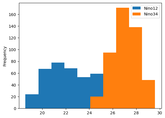
We can see some clear differences in the distributions, which is helpful! Another plot one might like to use would be a boxplot. Here, we replace hist with box
df[['Nino12', 'Nino34']].plot.box();
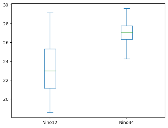
Here, we again see a clear difference in the distributions. These are not the only plots you can use within pandas! For more examples of plotting choices, check out the pandas plot documentation
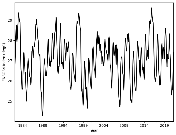
Customize your Plot
These plot() methods are just wrappers to matplotlib, so with a little more work the plots can be customized just like any matplotlib figure.
df.Nino34.plot(
    color='black',
    linewidth=2,
    xlabel='Year',
    ylabel='ENSO34 Index (degC)',
    figsize=(8, 6),
);
This can be a great way to take a quick look at your data, but what if you wanted a more quantitative perspective? We can use the describe method on our DataFrame; this returns a table of summary statistics for all columns in the DataFrame
Basic Statistics
By using the describe method, we see some general statistics! Notice how calling this on the dataframe returns a table with all the Series
df.describe()
| Nino12 | Nino12anom | Nino3 | Nino3anom | Nino4 | Nino4anom | Nino34 | Nino34anom | |
|---|---|---|---|---|---|---|---|---|
| count | 472.000000 | 472.000000 | 472.000000 | 472.000000 | 472.000000 | 472.000000 | 472.000000 | 472.000000 |
| mean | 23.209619 | 0.059725 | 25.936568 | 0.039428 | 28.625064 | 0.063814 | 27.076780 | 0.034894 |
| std | 2.431522 | 1.157590 | 1.349621 | 0.965464 | 0.755422 | 0.709401 | 1.063004 | 0.947936 |
| min | 18.570000 | -2.100000 | 23.030000 | -2.070000 | 26.430000 | -1.870000 | 24.270000 | -2.380000 |
| 25% | 21.152500 | -0.712500 | 24.850000 | -0.600000 | 28.140000 | -0.430000 | 26.330000 | -0.572500 |
| 50% | 22.980000 | -0.160000 | 25.885000 | -0.115000 | 28.760000 | 0.205000 | 27.100000 | 0.015000 |
| 75% | 25.322500 | 0.515000 | 26.962500 | 0.512500 | 29.190000 | 0.630000 | 27.792500 | 0.565000 |
| max | 29.150000 | 4.620000 | 29.140000 | 3.620000 | 30.300000 | 1.670000 | 29.600000 | 2.950000 |
You can look at specific statistics too, such as mean! Notice how the output is a Series (column) now
df.mean()
Nino12        23.209619
Nino12anom     0.059725
Nino3         25.936568
Nino3anom      0.039428
Nino4         28.625064
Nino4anom      0.063814
Nino34        27.076780
Nino34anom     0.034894
dtype: float64
If you are interested in a single column mean, subset for that and use .mean
df.Nino34.mean()
27.07677966101695
Subsetting Using the Datetime Column
You can use techniques besides slicing to subset a DataFrame. Here, we provide examples of using a couple other options.
Say you only want the month of January - you can use df.index.month to query for which month you are interested in (in this case, 1 for the month of January)
# Uses the datetime column
df[df.index.month == 1]
| Nino12 | Nino12anom | Nino3 | Nino3anom | Nino4 | Nino4anom | Nino34 | Nino34anom | |
|---|---|---|---|---|---|---|---|---|
| datetime | ||||||||
| 1982-01-01 | 24.29 | -0.17 | 25.87 | 0.24 | 28.30 | 0.00 | 26.72 | 0.15 |
| 1983-01-01 | 27.42 | 2.96 | 28.92 | 3.29 | 29.00 | 0.70 | 29.36 | 2.79 |
| 1984-01-01 | 24.18 | -0.28 | 24.82 | -0.81 | 27.64 | -0.66 | 25.64 | -0.93 |
| 1985-01-01 | 23.59 | -0.87 | 24.51 | -1.12 | 27.71 | -0.59 | 25.43 | -1.14 |
| 1986-01-01 | 24.61 | 0.15 | 24.73 | -0.90 | 28.11 | -0.19 | 25.79 | -0.78 |
| 1987-01-01 | 25.30 | 0.84 | 26.69 | 1.06 | 29.02 | 0.72 | 27.91 | 1.34 |
| 1988-01-01 | 24.64 | 0.18 | 26.12 | 0.49 | 29.13 | 0.83 | 27.32 | 0.75 |
| 1989-01-01 | 24.09 | -0.37 | 24.15 | -1.48 | 26.54 | -1.76 | 24.53 | -2.04 |
| 1990-01-01 | 24.02 | -0.44 | 25.34 | -0.29 | 28.56 | 0.26 | 26.55 | -0.02 |
| 1991-01-01 | 23.86 | -0.60 | 25.65 | 0.02 | 29.00 | 0.70 | 27.01 | 0.44 |
| 1992-01-01 | 24.83 | 0.37 | 27.00 | 1.37 | 29.06 | 0.76 | 28.41 | 1.84 |
| 1993-01-01 | 24.43 | -0.03 | 25.56 | -0.07 | 28.60 | 0.30 | 26.69 | 0.12 |
| 1994-01-01 | 24.32 | -0.14 | 25.71 | 0.08 | 28.47 | 0.17 | 26.60 | 0.03 |
| 1995-01-01 | 25.33 | 0.87 | 26.34 | 0.71 | 29.20 | 0.90 | 27.55 | 0.98 |
| 1996-01-01 | 23.84 | -0.62 | 24.96 | -0.67 | 27.92 | -0.38 | 25.74 | -0.83 |
| 1997-01-01 | 23.67 | -0.79 | 24.70 | -0.93 | 28.41 | 0.11 | 25.96 | -0.61 |
| 1998-01-01 | 28.22 | 3.76 | 28.94 | 3.31 | 29.01 | 0.71 | 29.10 | 2.53 |
| 1999-01-01 | 23.73 | -0.73 | 24.41 | -1.22 | 26.59 | -1.71 | 24.90 | -1.67 |
| 2000-01-01 | 23.86 | -0.60 | 23.88 | -1.75 | 26.96 | -1.34 | 24.65 | -1.92 |
| 2001-01-01 | 23.88 | -0.58 | 24.99 | -0.64 | 27.50 | -0.80 | 25.74 | -0.83 |
| 2002-01-01 | 23.64 | -0.82 | 25.09 | -0.54 | 28.81 | 0.51 | 26.50 | -0.07 |
| 2003-01-01 | 24.38 | -0.08 | 26.38 | 0.75 | 29.25 | 0.95 | 27.76 | 1.19 |
| 2004-01-01 | 24.60 | 0.14 | 25.92 | 0.29 | 28.83 | 0.53 | 26.74 | 0.17 |
| 2005-01-01 | 24.47 | 0.01 | 25.89 | 0.26 | 29.21 | 0.91 | 27.10 | 0.53 |
| 2006-01-01 | 24.33 | -0.13 | 25.00 | -0.63 | 27.68 | -0.62 | 25.64 | -0.93 |
| 2007-01-01 | 24.99 | 0.53 | 26.50 | 0.87 | 28.93 | 0.63 | 27.26 | 0.69 |
| 2008-01-01 | 23.86 | -0.60 | 24.13 | -1.50 | 26.62 | -1.68 | 24.71 | -1.86 |
| 2009-01-01 | 24.42 | -0.10 | 25.03 | -0.60 | 27.42 | -0.88 | 25.54 | -1.03 |
| 2010-01-01 | 24.82 | 0.30 | 26.63 | 1.00 | 29.51 | 1.21 | 28.07 | 1.50 |
| 2011-01-01 | 24.08 | -0.44 | 24.31 | -1.32 | 26.72 | -1.58 | 24.93 | -1.64 |
| 2012-01-01 | 23.88 | -0.64 | 24.90 | -0.73 | 27.09 | -1.21 | 25.49 | -1.08 |
| 2013-01-01 | 24.00 | -0.52 | 25.06 | -0.57 | 28.28 | -0.02 | 26.16 | -0.41 |
| 2014-01-01 | 24.79 | 0.27 | 25.26 | -0.37 | 28.14 | -0.17 | 26.06 | -0.51 |
| 2015-01-01 | 24.13 | -0.39 | 25.99 | 0.36 | 29.16 | 0.86 | 27.10 | 0.53 |
| 2016-01-01 | 25.93 | 1.41 | 28.21 | 2.58 | 29.65 | 1.35 | 29.17 | 2.60 |
| 2017-01-01 | 25.75 | 1.23 | 25.61 | -0.02 | 28.18 | -0.12 | 26.25 | -0.32 |
| 2018-01-01 | 23.71 | -0.81 | 24.48 | -1.14 | 28.03 | -0.27 | 25.82 | -0.75 |
| 2019-01-01 | 25.10 | 0.57 | 26.17 | 0.55 | 29.00 | 0.65 | 27.08 | 0.52 |
| 2020-01-01 | 24.55 | 0.02 | 25.81 | 0.20 | 29.28 | 0.93 | 27.09 | 0.53 |
| 2021-01-01 | 23.89 | -0.64 | 25.06 | -0.55 | 27.10 | -1.25 | 25.58 | -0.99 |
You could even assign this month to a new column!
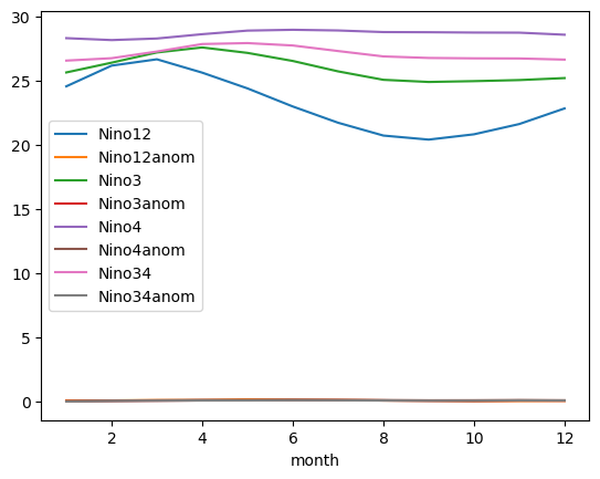
df['month'] = df.index.month
Now that it is its own column (Series), we can use groupby to group by the month, then taking the average, to determine average monthly values over the dataset
df.groupby('month').mean().plot();
Investigating Extreme Values
You can also use conditional indexing, such that you can search where rows meet a certain criteria. In this case, we are interested in where the Nino34 anomaly is greater than 2
df[df.Nino34anom > 2]
| Nino12 | Nino12anom | Nino3 | Nino3anom | Nino4 | Nino4anom | Nino34 | Nino34anom | month | |
|---|---|---|---|---|---|---|---|---|---|
| datetime | |||||||||
| 1982-11-01 | 24.59 | 3.00 | 27.62 | 2.64 | 29.23 | 0.60 | 28.81 | 2.16 | 11 |
| 1982-12-01 | 26.13 | 3.34 | 28.39 | 3.25 | 29.15 | 0.66 | 29.21 | 2.64 | 12 |
| 1983-01-01 | 27.42 | 2.96 | 28.92 | 3.29 | 29.00 | 0.70 | 29.36 | 2.79 | 1 |
| 1983-02-01 | 28.09 | 2.02 | 28.92 | 2.55 | 28.79 | 0.69 | 29.13 | 2.41 | 2 |
| 1997-08-01 | 24.80 | 4.15 | 27.84 | 2.85 | 29.26 | 0.58 | 28.84 | 2.02 | 8 |
| 1997-09-01 | 24.40 | 4.04 | 27.84 | 2.99 | 29.32 | 0.63 | 28.93 | 2.21 | 9 |
| 1997-10-01 | 24.58 | 3.76 | 28.17 | 3.25 | 29.32 | 0.66 | 29.23 | 2.54 | 10 |
| 1997-11-01 | 25.63 | 4.04 | 28.55 | 3.57 | 29.49 | 0.86 | 29.32 | 2.67 | 11 |
| 1997-12-01 | 26.92 | 4.13 | 28.76 | 3.62 | 29.32 | 0.83 | 29.26 | 2.69 | 12 |
| 1998-01-01 | 28.22 | 3.76 | 28.94 | 3.31 | 29.01 | 0.71 | 29.10 | 2.53 | 1 |
| 1998-02-01 | 28.98 | 2.91 | 28.93 | 2.56 | 28.87 | 0.77 | 28.86 | 2.14 | 2 |
| 2015-08-01 | 22.88 | 2.24 | 27.33 | 2.34 | 29.66 | 0.98 | 28.89 | 2.07 | 8 |
| 2015-09-01 | 22.91 | 2.57 | 27.48 | 2.63 | 29.73 | 1.04 | 29.00 | 2.28 | 9 |
| 2015-10-01 | 23.31 | 2.52 | 27.58 | 2.66 | 29.79 | 1.12 | 29.15 | 2.46 | 10 |
| 2015-11-01 | 23.83 | 2.24 | 27.91 | 2.93 | 30.30 | 1.67 | 29.60 | 2.95 | 11 |
| 2015-12-01 | 25.01 | 2.19 | 27.99 | 2.85 | 30.11 | 1.63 | 29.39 | 2.82 | 12 |
| 2016-01-01 | 25.93 | 1.41 | 28.21 | 2.58 | 29.65 | 1.35 | 29.17 | 2.60 | 1 |
| 2016-02-01 | 26.81 | 0.67 | 28.36 | 1.99 | 29.55 | 1.45 | 29.12 | 2.40 | 2 |
You can also sort columns based on the values!
df.sort_values('Nino34anom')
| Nino12 | Nino12anom | Nino3 | Nino3anom | Nino4 | Nino4anom | Nino34 | Nino34anom | month | |
|---|---|---|---|---|---|---|---|---|---|
| datetime | |||||||||
| 1988-11-01 | 20.55 | -1.04 | 23.03 | -1.95 | 26.76 | -1.87 | 24.27 | -2.38 | 11 |
| 1988-12-01 | 21.80 | -0.99 | 23.07 | -2.07 | 26.75 | -1.74 | 24.33 | -2.24 | 12 |
| 1988-10-01 | 19.50 | -1.32 | 23.17 | -1.75 | 27.06 | -1.60 | 24.62 | -2.07 | 10 |
| 1989-01-01 | 24.09 | -0.37 | 24.15 | -1.48 | 26.54 | -1.76 | 24.53 | -2.04 | 1 |
| 2000-01-01 | 23.86 | -0.60 | 23.88 | -1.75 | 26.96 | -1.34 | 24.65 | -1.92 | 1 |
| ... | ... | ... | ... | ... | ... | ... | ... | ... | ... |
| 1997-11-01 | 25.63 | 4.04 | 28.55 | 3.57 | 29.49 | 0.86 | 29.32 | 2.67 | 11 |
| 1997-12-01 | 26.92 | 4.13 | 28.76 | 3.62 | 29.32 | 0.83 | 29.26 | 2.69 | 12 |
| 1983-01-01 | 27.42 | 2.96 | 28.92 | 3.29 | 29.00 | 0.70 | 29.36 | 2.79 | 1 |
| 2015-12-01 | 25.01 | 2.19 | 27.99 | 2.85 | 30.11 | 1.63 | 29.39 | 2.82 | 12 |
| 2015-11-01 | 23.83 | 2.24 | 27.91 | 2.93 | 30.30 | 1.67 | 29.60 | 2.95 | 11 |
472 rows × 9 columns
Let’s change the way that is ordered…
df.sort_values('Nino34anom', ascending=False)
| Nino12 | Nino12anom | Nino3 | Nino3anom | Nino4 | Nino4anom | Nino34 | Nino34anom | month | |
|---|---|---|---|---|---|---|---|---|---|
| datetime | |||||||||
| 2015-11-01 | 23.83 | 2.24 | 27.91 | 2.93 | 30.30 | 1.67 | 29.60 | 2.95 | 11 |
| 2015-12-01 | 25.01 | 2.19 | 27.99 | 2.85 | 30.11 | 1.63 | 29.39 | 2.82 | 12 |
| 1983-01-01 | 27.42 | 2.96 | 28.92 | 3.29 | 29.00 | 0.70 | 29.36 | 2.79 | 1 |
| 1997-12-01 | 26.92 | 4.13 | 28.76 | 3.62 | 29.32 | 0.83 | 29.26 | 2.69 | 12 |
| 1997-11-01 | 25.63 | 4.04 | 28.55 | 3.57 | 29.49 | 0.86 | 29.32 | 2.67 | 11 |
| ... | ... | ... | ... | ... | ... | ... | ... | ... | ... |
| 2000-01-01 | 23.86 | -0.60 | 23.88 | -1.75 | 26.96 | -1.34 | 24.65 | -1.92 | 1 |
| 1989-01-01 | 24.09 | -0.37 | 24.15 | -1.48 | 26.54 | -1.76 | 24.53 | -2.04 | 1 |
| 1988-10-01 | 19.50 | -1.32 | 23.17 | -1.75 | 27.06 | -1.60 | 24.62 | -2.07 | 10 |
| 1988-12-01 | 21.80 | -0.99 | 23.07 | -2.07 | 26.75 | -1.74 | 24.33 | -2.24 | 12 |
| 1988-11-01 | 20.55 | -1.04 | 23.03 | -1.95 | 26.76 | -1.87 | 24.27 | -2.38 | 11 |
472 rows × 9 columns
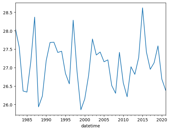
Resampling
Here, we are trying to resample the timeseries such that the signal does not appear as noisy. This can helpfule when working with timeseries data! In this case, we resample to a yearly average (1Y) instead of monthly values
df.Nino34.plot();
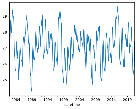
df.Nino34.resample('1Y').mean().plot();
Applying operations to a dataframe
Often times, people are interested in applying calculations to data within pandas DataFrames. Here, we setup a function to convert from degrees Celsius to Kelvin
def convert_degc_to_kelvin(temperature_degc):
    """
    Converts from degrees celsius to Kelvin
    """

    return temperature_degc + 273.15
Now, this function accepts and returns a single value
# Convert a single value
convert_degc_to_kelvin(0)
273.15
But what if we want to apply this to our dataframe? We can subset for Nino34, which is in degrees Celsius
nino34_series
datetime
1982-01-01    26.72
1982-02-01    26.70
1982-03-01    27.20
1982-04-01    28.02
1982-05-01    28.54
              ...
2020-12-01    25.53
2021-01-01    25.58
2021-02-01    25.81
2021-03-01    26.75
2021-04-01    27.40
Name: Nino34, Length: 472, dtype: float64
Notice how the object type is a pandas series
type(df.Nino12[0:10])
pandas.core.series.Series
If you call .values, the object type is now a numpy array. Pandas Series values include numpy arrays, and calling .values returns the series as a numpy array!
type(df.Nino12.values[0:10])
numpy.ndarray
Let’s apply this calculation to this Series; this returns another Series object.
convert_degc_to_kelvin(nino34_series)
datetime
1982-01-01    299.87
1982-02-01    299.85
1982-03-01    300.35
1982-04-01    301.17
1982-05-01    301.69
               ...
2020-12-01    298.68
2021-01-01    298.73
2021-02-01    298.96
2021-03-01    299.90
2021-04-01    300.55
Name: Nino34, Length: 472, dtype: float64
If we include .values, it returns a numpy array
Warning
We don’t usually recommend converting to NumPy arrays unless you need to - once you convert to NumPy arrays, the helpful label information is lost… so beware!
convert_degc_to_kelvin(nino34_series.values)
array([299.87, 299.85, 300.35, 301.17, 301.69, 301.9 , 301.25, 301.08,
       301.26, 301.79, 301.96, 302.36, 302.51, 302.28, 302.18, 302.06,
       302.04, 301.39, 300.22, 299.68, 299.59, 299.02, 298.73, 298.74,
       298.79, 299.54, 300.01, 300.54, 300.54, 300.01, 299.89, 299.49,
       299.58, 299.08, 298.56, 298.15, 298.58, 298.82, 299.38, 299.95,
       300.26, 300.01, 299.84, 299.65, 299.4 , 299.34, 299.34, 299.26,
       298.94, 299.09, 299.8 , 300.59, 300.65, 300.84, 300.52, 300.3 ,
       300.48, 300.72, 300.88, 300.85, 301.06, 301.17, 301.62, 301.95,
       301.9 , 302.18, 301.95, 301.73, 301.54, 301.22, 301.14, 300.75,
       300.47, 300.37, 300.46, 300.47, 299.63, 299.26, 298.72, 298.39,
       298.58, 297.77, 297.42, 297.48, 297.68, 298.48, 299.05, 299.84,
       300.24, 300.13, 299.89, 299.48, 299.4 , 299.41, 299.39, 299.53,
       299.7 , 300.1 , 300.61, 301.17, 301.21, 300.73, 300.4 , 300.2 ,
       299.9 , 300.13, 299.87, 300.06, 300.16, 300.08, 300.4 , 301.13,
       301.5 , 301.51, 301.07, 300.59, 300.22, 300.78, 301.01, 301.52,
       301.56, 301.78, 301.98, 302.29, 302.14, 301.17, 300.68, 299.79,
       299.63, 299.49, 299.66, 299.88, 299.84, 300.12, 300.81, 301.74,
       301.97, 301.43, 300.7 , 299.99, 300.07, 300.08, 300.06, 299.91,
       299.75, 299.74, 300.42, 301.05, 301.19, 301.14, 300.5 , 300.5 ,
       300.15, 300.64, 301.02, 301.02, 300.7 , 300.6 , 300.78, 301.08,
       300.88, 300.74, 300.16, 299.48, 299.11, 298.82, 298.81, 298.72,
       298.89, 299.  , 299.77, 300.51, 300.52, 300.47, 300.24, 299.71,
       299.5 , 299.39, 299.34, 299.17, 299.11, 299.51, 300.18, 301.18,
       301.75, 302.09, 302.07, 301.99, 302.08, 302.38, 302.47, 302.41,
       302.25, 302.01, 301.82, 301.71, 301.62, 299.87, 299.09, 298.64,
       298.76, 298.49, 298.33, 297.94, 298.05, 298.56, 299.4 , 299.99,
       300.12, 299.75, 299.5 , 298.74, 298.86, 298.79, 298.27, 298.05,
       297.8 , 298.34, 299.23, 300.16, 300.27, 300.18, 299.87, 299.6 ,
       299.36, 299.11, 298.93, 298.74, 298.89, 299.26, 299.99, 300.67,
       300.75, 300.83, 300.47, 300.02, 299.7 , 299.74, 299.6 , 299.32,
       299.65, 300.1 , 300.47, 301.09, 301.3 , 301.58, 301.13, 300.94,
       300.98, 301.2 , 301.42, 301.24, 300.91, 300.64, 300.96, 300.96,
       300.52, 300.63, 300.58, 300.  , 300.11, 300.34, 300.2 , 300.04,
       299.89, 300.01, 300.25, 300.99, 301.21, 300.91, 300.84, 300.69,
       300.62, 300.53, 300.46, 300.46, 300.25, 300.11, 300.7 , 301.22,
       301.35, 301.2 , 300.62, 300.03, 299.78, 299.9 , 299.49, 299.04,
       298.79, 299.23, 299.72, 300.74, 301.06, 301.  , 300.5 , 300.37,
       300.49, 300.62, 300.88, 300.91, 300.41, 299.96, 300.33, 300.93,
       300.72, 300.7 , 299.94, 299.35, 298.92, 298.37, 298.21, 298.12,
       297.86, 297.98, 299.22, 299.98, 300.33, 300.32, 300.34, 300.  ,
       299.59, 299.48, 299.45, 298.89, 298.69, 299.19, 299.82, 300.65,
       301.18, 301.26, 301.09, 300.68, 300.62, 300.78, 301.34, 301.45,
       301.22, 301.09, 301.44, 301.51, 300.83, 300.15, 299.24, 298.65,
       298.22, 298.16, 298.22, 298.1 , 298.08, 298.61, 299.38, 300.17,
       300.57, 300.61, 300.11, 299.34, 299.13, 298.87, 298.75, 298.68,
       298.64, 299.18, 299.78, 300.53, 300.95, 301.1 , 300.9 , 300.7 ,
       300.39, 300.13, 300.16, 299.61, 299.31, 299.47, 300.15, 300.83,
       300.72, 300.58, 300.06, 299.69, 299.8 , 299.51, 299.8 , 299.68,
       299.21, 299.33, 300.14, 301.16, 301.46, 301.26, 300.55, 300.17,
       300.32, 300.32, 300.65, 300.5 , 300.25, 300.44, 300.94, 301.71,
       302.03, 302.11, 301.97, 302.04, 302.15, 302.3 , 302.75, 302.54,
       302.32, 302.27, 302.05, 302.02, 301.3 , 300.68, 299.88, 299.43,
       299.26, 299.11, 299.25, 299.31, 299.4 , 300.02, 300.49, 301.25,
       301.45, 301.34, 300.76, 299.82, 299.44, 299.38, 298.94, 298.95,
       298.97, 298.98, 299.63, 300.57, 300.87, 301.  , 300.67, 300.26,
       300.25, 300.7 , 300.79, 300.68, 300.23, 300.56, 301.37, 301.75,
       301.72, 301.39, 300.78, 300.12, 299.85, 300.46, 300.41, 300.22,
       300.24, 300.29, 300.97, 301.47, 300.74, 300.45, 300.04, 299.33,
       298.92, 298.45, 298.49, 298.68, 298.73, 298.96, 299.9 , 300.55])
We can now assign our pandas Series with the converted temperatures to a new column in our dataframe!
df['Nino34_degK'] = convert_degc_to_kelvin(nino34_series)
df.Nino34_degK
datetime
1982-01-01    299.87
1982-02-01    299.85
1982-03-01    300.35
1982-04-01    301.17
1982-05-01    301.69
               ...
2020-12-01    298.68
2021-01-01    298.73
2021-02-01    298.96
2021-03-01    299.90
2021-04-01    300.55
Name: Nino34_degK, Length: 472, dtype: float64
Now that our analysis is done, we can save our data to a csv for later - or share with others!
df.to_csv('nino_analyzed_output.csv')
pd.read_csv('nino_analyzed_output.csv', index_col=0, parse_dates=True)
| Nino12 | Nino12anom | Nino3 | Nino3anom | Nino4 | Nino4anom | Nino34 | Nino34anom | month | Nino34_degK | |
|---|---|---|---|---|---|---|---|---|---|---|
| datetime | ||||||||||
| 1982-01-01 | 24.29 | -0.17 | 25.87 | 0.24 | 28.30 | 0.00 | 26.72 | 0.15 | 1 | 299.87 |
| 1982-02-01 | 25.49 | -0.58 | 26.38 | 0.01 | 28.21 | 0.11 | 26.70 | -0.02 | 2 | 299.85 |
| 1982-03-01 | 25.21 | -1.31 | 26.98 | -0.16 | 28.41 | 0.22 | 27.20 | -0.02 | 3 | 300.35 |
| 1982-04-01 | 24.50 | -0.97 | 27.68 | 0.18 | 28.92 | 0.42 | 28.02 | 0.24 | 4 | 301.17 |
| 1982-05-01 | 23.97 | -0.23 | 27.79 | 0.71 | 29.49 | 0.70 | 28.54 | 0.69 | 5 | 301.69 |
| ... | ... | ... | ... | ... | ... | ... | ... | ... | ... | ... |
| 2020-12-01 | 22.16 | -0.60 | 24.38 | -0.83 | 27.65 | -0.95 | 25.53 | -1.12 | 12 | 298.68 |
| 2021-01-01 | 23.89 | -0.64 | 25.06 | -0.55 | 27.10 | -1.25 | 25.58 | -0.99 | 1 | 298.73 |
| 2021-02-01 | 25.55 | -0.66 | 25.80 | -0.57 | 27.20 | -1.00 | 25.81 | -0.92 | 2 | 298.96 |
| 2021-03-01 | 26.48 | -0.26 | 26.80 | -0.39 | 27.79 | -0.55 | 26.75 | -0.51 | 3 | 299.90 |
| 2021-04-01 | 24.89 | -0.80 | 26.96 | -0.65 | 28.47 | -0.21 | 27.40 | -0.49 | 4 | 300.55 |
472 rows × 10 columns
Summary
Pandas is a very powerful tool for working with tabular (i.e. spreadsheet-style) data
There are multiple ways of subsetting your pandas dataframe or series
Pandas allows you to refer to subsets of data by label, which generally makes code more readable and more robust
Pandas can be helpful for exploratory data analysis, including plotting and basic statistics
One can apply calculations to pandas dataframes and save the output via
csvfiles