
Dask Arrays with Xarray
Dask array provides a parallel, larger-than-memory, n-dimensional array using blocked algorithms. Simply put: distributed Numpy.
Parallel: Uses all of the cores on your computer
Larger-than-memory: Lets you work on datasets that are larger than your available memory by breaking up your array into many small pieces, operating on those pieces in an order that minimizes the memory footprint of your computation, and effectively streaming data from disk.
Blocked Algorithms: Perform large computations by performing many smaller computations
This notebook demonstrates one of Xarray’s most powerful features: the ability to wrap dask arrays and allow users to seamlessly execute analysis code in parallel.
Learning Objectives
Understand key features of dask arrays
Work with Dask Array’s in much the same way you would work with a NumPy array
Learn that xarray DataArrays and Datasets are “dask collections” i.e. you can execute top-level dask functions such as dask.visualize(xarray_object)
Learn that all xarray built-in operations can transparently use dask
Prerequisites
Concepts |
Importance |
Notes |
|---|---|---|
Familiarity with NumPy |
Necessary |
|
Familiarity with Xarray |
Necessary |
Time to learn: 30-40 minutes
Imports
import dask
import dask.array as da
import numpy as np
import xarray as xr
from dask.diagnostics import ProgressBar
from dask.utils import format_bytes
from pythia_datasets import DATASETS
Blocked algorithms
A blocked algorithm executes on a large dataset by breaking it up into many small blocks.
For example, consider taking the sum of a billion numbers, in a single computation. This would take a while. We might instead break up the array into 1,000 chunks, each of size 1,000,000, take the sum of each chunk, and then take the sum of the intermediate sums.
We achieve the intended result (one sum on one billion numbers) by performing many smaller results (one thousand sums on one million numbers each, followed by another sum of a thousand numbers.)
dask.array contains these algorithms
dask.array implements a subset of the NumPy ndarray interface using blocked algorithms, cutting up the large array into many small arrays. This lets us compute on arrays larger than memory using multiple cores. We coordinate these blocked algorithms using Dask graphs. Dask Array’s are also lazy, meaning that they do not evaluate until you explicitly ask for a result using the compute method.
Create a dask.array object
If we want to create a 3D NumPy array of random values, we do it like this:
shape = (600, 200, 200)
arr = np.random.random(shape)
arr
array([[[0.49822623, 0.83109134, 0.06873832, ..., 0.48004661,
         0.1154805 , 0.40895164],
        [0.05860555, 0.47832112, 0.67367543, ..., 0.11818103,
         0.36086032, 0.60881463],
        [0.64280277, 0.31653276, 0.72027114, ..., 0.72299986,
         0.10866501, 0.80298659],
        ...,
        [0.50049719, 0.69705375, 0.82471421, ..., 0.0794366 ,
         0.85967716, 0.51323268],
        [0.59051297, 0.87904695, 0.77321564, ..., 0.70236725,
         0.70568836, 0.2366349 ],
        [0.60761527, 0.54185241, 0.51628965, ..., 0.4786314 ,
         0.23286647, 0.66406195]],

       [[0.36076331, 0.33318767, 0.15614146, ..., 0.64147273,
         0.37413077, 0.4786213 ],
        [0.37262609, 0.81957454, 0.60755709, ..., 0.18336461,
         0.83839824, 0.86669838],
        [0.42277283, 0.66374626, 0.76158239, ..., 0.55970321,
         0.59111663, 0.75437946],
        ...,
        [0.39564903, 0.24109262, 0.66964801, ..., 0.28883724,
         0.71008329, 0.28667933],
        [0.96354285, 0.17278661, 0.10031896, ..., 0.6339706 ,
         0.26528233, 0.39969547],
        [0.86832276, 0.97531806, 0.02650584, ..., 0.66453284,
         0.57126407, 0.00868137]],

       [[0.81306258, 0.82725182, 0.60773151, ..., 0.91856456,
         0.45240577, 0.08321277],
        [0.42541671, 0.46525316, 0.06807218, ..., 0.25537894,
         0.52327985, 0.40055532],
        [0.73956505, 0.01708811, 0.28872035, ..., 0.78020928,
         0.33996816, 0.85454659],
        ...,
        [0.9533748 , 0.43850099, 0.14844177, ..., 0.11396482,
         0.03550981, 0.90763319],
        [0.75357982, 0.13804137, 0.63610922, ..., 0.86628727,
         0.31668596, 0.60421854],
        [0.30627269, 0.1696831 , 0.30264352, ..., 0.67914138,
         0.96485397, 0.55254373]],

       ...,

       [[0.99444642, 0.79261704, 0.78733796, ..., 0.63640423,
         0.94784652, 0.24173185],
        [0.15809555, 0.34361539, 0.64785782, ..., 0.22990406,
         0.74957486, 0.87113614],
        [0.20614992, 0.42170253, 0.21391395, ..., 0.71304801,
         0.13376829, 0.98317853],
        ...,
        [0.22690905, 0.27102062, 0.93863401, ..., 0.52797775,
         0.25255965, 0.76361088],
        [0.73692766, 0.13837857, 0.12689666, ..., 0.10825688,
         0.39841364, 0.54760738],
        [0.77950787, 0.42836872, 0.70157517, ..., 0.40836473,
         0.11879859, 0.97832284]],

       [[0.37544966, 0.21529608, 0.30190067, ..., 0.77315465,
         0.01750085, 0.00776369],
        [0.88533243, 0.33808008, 0.58628251, ..., 0.21418   ,
         0.79270547, 0.52502577],
        [0.52932151, 0.39742119, 0.5584329 , ..., 0.23120074,
         0.23980939, 0.76846219],
        ...,
        [0.31176722, 0.38426033, 0.38627884, ..., 0.79444079,
         0.68591162, 0.39910299],
        [0.13532854, 0.66262792, 0.35416999, ..., 0.03306294,
         0.85574073, 0.92065125],
        [0.11917685, 0.88913219, 0.49048526, ..., 0.89476855,
         0.09888746, 0.78118624]],

       [[0.9543262 , 0.33891494, 0.05249305, ..., 0.78558061,
         0.51634066, 0.20669244],
        [0.29947346, 0.6708223 , 0.7334545 , ..., 0.67246413,
         0.45671407, 0.12259186],
        [0.77647366, 0.58799202, 0.16516736, ..., 0.83749073,
         0.22535282, 0.74740628],
        ...,
        [0.27432374, 0.33545776, 0.69337022, ..., 0.63016243,
         0.11684087, 0.06671004],
        [0.48981101, 0.79523335, 0.47443195, ..., 0.38062945,
         0.91165591, 0.93456084],
        [0.30744634, 0.12745334, 0.64803194, ..., 0.82943371,
         0.09908842, 0.67925487]]])
format_bytes(arr.nbytes)
'183.11 MiB'
This array contains ~183 MB of data
Now let’s create the same array using Dask’s array interface.
darr = da.random.random(shape, chunks=(300, 100, 200))
A chunk size to tell us how to block up our array, like (300, 100, 200).
Specifying Chunks
There are several ways to specify chunks. In this tutorial, we will use a block shape.
darr
|
||||||||||||||||
Notice that we just see a symbolic representation of the array, including its shape, dtype, and chunksize. No data has been generated yet. Let’s visualize the constructed task graph.
darr.visualize()
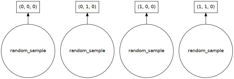
Our array has four chunks. To generate it, Dask calls np.random.random four times and then concatenates this together into one array.
Manipulate a dask.array object as you would a numpy array
Now that we have an Array we perform standard numpy-style computations like arithmetic, mathematics, slicing, reductions, etc…
The interface is familiar, but the actual work is different. dask_array.sum() does not do the same thing as numpy_array.sum().
What’s the difference?
dask_array.sum() builds an expression of the computation. It does not do the computation yet. numpy_array.sum() computes the sum immediately.
Why the difference?
Dask arrays are split into chunks. Each chunk must have computations run on that chunk explicitly. If the desired answer comes from a small slice of the entire dataset, running the computation over all data would be wasteful of CPU and memory.
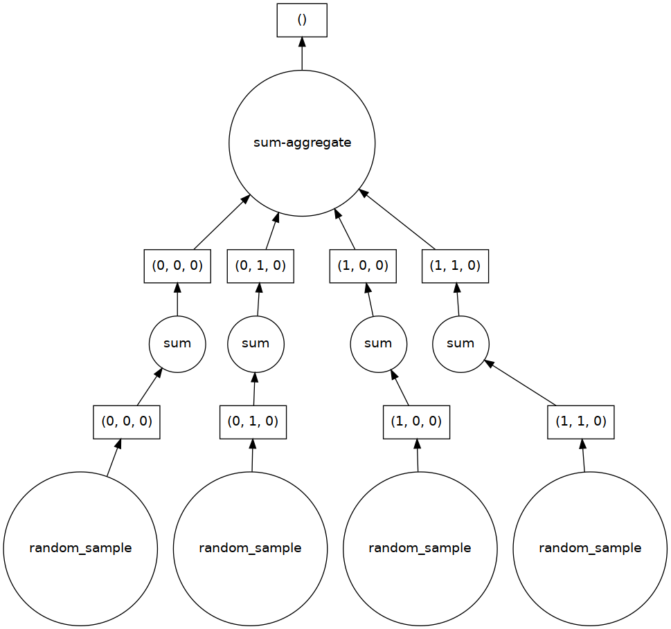
total = darr.sum()
total
|
||||||||||||||||
total.visualize()
Compute the result
Dask.array objects are lazily evaluated. Operations like .sum build up a graph of blocked tasks to execute.
We ask for the final result with a call to .compute(). This triggers the actual computation.
%%time
total.compute()
CPU times: user 242 ms, sys: 83.5 ms, total: 325 ms
Wall time: 187 ms
11998546.555704407
Exercise with dask.arrays
Modify the chunk size (or shape) in the random dask array, call .sum() on the new array, and visualize how the task graph changes.
da.random.random(shape, chunks=(50, 200, 400)).sum().visualize()
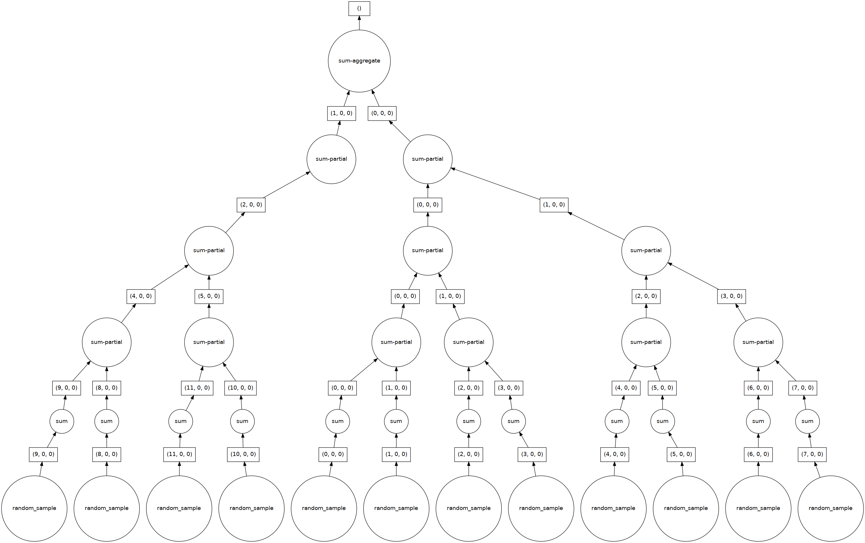
Here we see Dask’s strategy for finding the sum. This simple example illustrates the beauty of Dask: it automatically designs an algorithm appropriate for custom operations with big data.
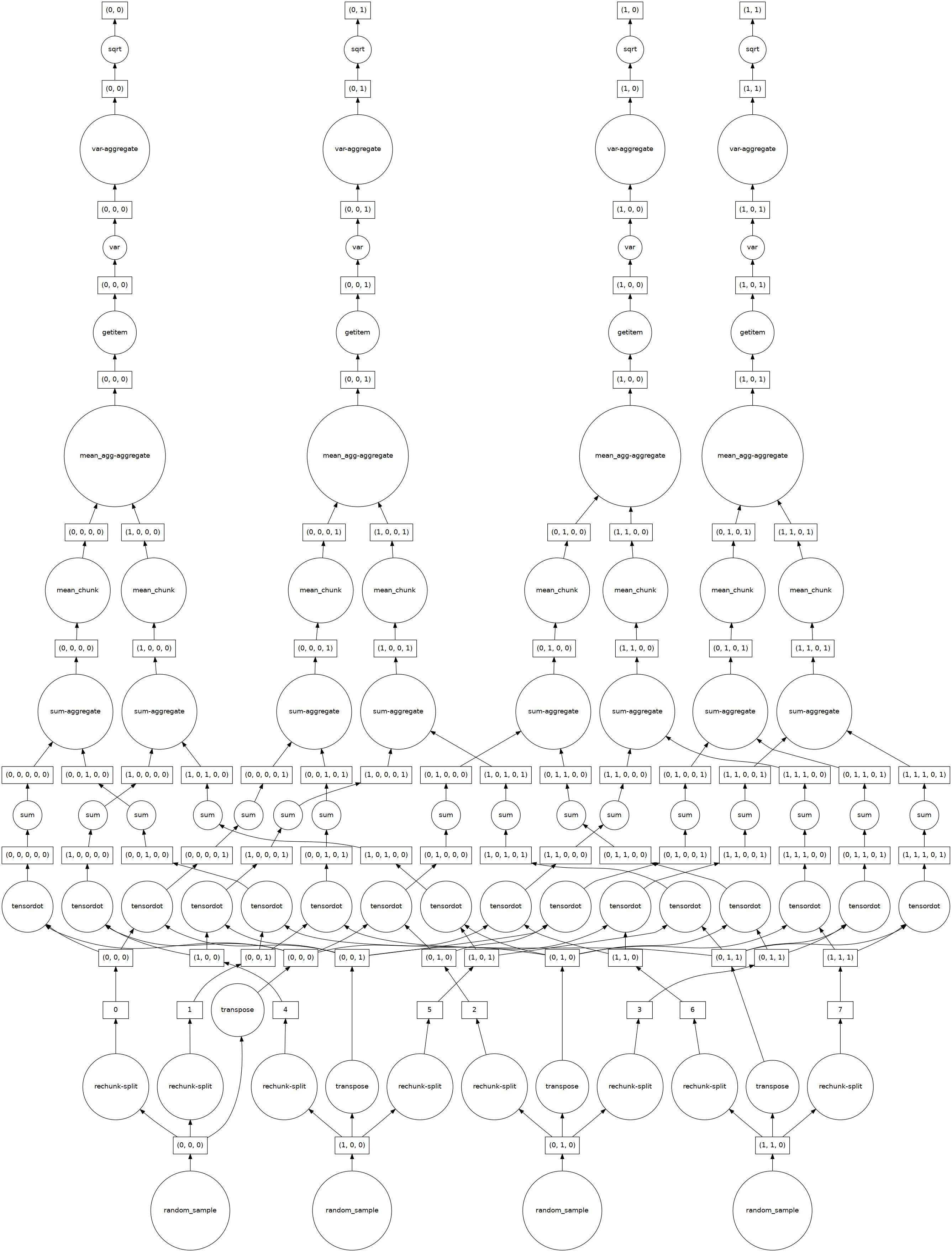
If we make our operation more complex, the graph gets more complex:
z = darr.dot(darr.T).mean(axis=0)[::2, :].std(axis=1)
z
|
||||||||||||||||
z.visualize()
Testing a bigger calculation
The examples above were toy examples; the data (180 MB) is probably not big enough to warrant the use of Dask.
We can make it a lot bigger! Let’s create a new, big array
darr = da.random.random((4000, 100, 4000), chunks=(1000, 100, 500)).astype('float32')
darr
|
||||||||||||||||
This dataset is ~6 GB, rather than 32 MB! This is probably close to or greater than the amount of available RAM than you have in your computer. Nevertheless, Dask has no problem working on it.
z = (darr + darr.T)[::2, :].mean(axis=2)
z.visualize()
with ProgressBar():
    computed_ds = z.compute()
[ ] | 0% Completed | 377.23 us
[ ] | 0% Completed | 108.57 ms
[ ] | 0% Completed | 209.73 ms
[ ] | 0% Completed | 310.83 ms
[ ] | 0% Completed | 411.89 ms
[ ] | 0% Completed | 514.20 ms
[ ] | 0% Completed | 616.43 ms
[ ] | 0% Completed | 718.20 ms
[ ] | 0% Completed | 821.69 ms
[ ] | 0% Completed | 924.04 ms
[ ] | 0% Completed | 1.03 s
[ ] | 0% Completed | 1.13 s
[ ] | 0% Completed | 1.23 s
[ ] | 1% Completed | 1.34 s
[ ] | 1% Completed | 1.44 s
[ ] | 1% Completed | 1.54 s
[# ] | 2% Completed | 1.65 s
[# ] | 2% Completed | 1.75 s
[# ] | 2% Completed | 1.85 s
[# ] | 3% Completed | 1.95 s
[# ] | 3% Completed | 2.05 s
[## ] | 5% Completed | 2.15 s
[## ] | 5% Completed | 2.25 s
[## ] | 5% Completed | 2.36 s
[## ] | 5% Completed | 2.46 s
[## ] | 5% Completed | 2.56 s
[## ] | 5% Completed | 2.66 s
[## ] | 5% Completed | 2.76 s
[## ] | 5% Completed | 2.86 s
[## ] | 6% Completed | 2.96 s
[### ] | 7% Completed | 3.06 s
[### ] | 8% Completed | 3.17 s
[### ] | 9% Completed | 3.27 s
[### ] | 9% Completed | 3.37 s
[#### ] | 10% Completed | 3.47 s
[#### ] | 11% Completed | 3.57 s
[#### ] | 11% Completed | 3.67 s
[#### ] | 11% Completed | 3.77 s
[#### ] | 11% Completed | 3.87 s
[#### ] | 11% Completed | 3.97 s
[#### ] | 11% Completed | 4.07 s
[#### ] | 11% Completed | 4.18 s
[#### ] | 11% Completed | 4.28 s
[#### ] | 11% Completed | 4.38 s
[##### ] | 13% Completed | 4.48 s
[##### ] | 13% Completed | 4.58 s
[##### ] | 14% Completed | 4.68 s
[###### ] | 15% Completed | 4.78 s
[###### ] | 15% Completed | 4.88 s
[###### ] | 15% Completed | 4.98 s
[###### ] | 16% Completed | 5.09 s
[###### ] | 16% Completed | 5.19 s
[###### ] | 16% Completed | 5.29 s
[###### ] | 16% Completed | 5.39 s
[###### ] | 16% Completed | 5.50 s
[###### ] | 16% Completed | 5.60 s
[###### ] | 16% Completed | 5.70 s
[###### ] | 16% Completed | 5.80 s
[###### ] | 16% Completed | 5.91 s
[###### ] | 16% Completed | 6.01 s
[###### ] | 16% Completed | 6.12 s
[####### ] | 18% Completed | 6.23 s
[####### ] | 19% Completed | 6.33 s
[####### ] | 19% Completed | 6.43 s
[####### ] | 19% Completed | 6.53 s
[######## ] | 21% Completed | 6.63 s
[######## ] | 21% Completed | 6.74 s
[######## ] | 21% Completed | 6.84 s
[######## ] | 22% Completed | 6.94 s
[######## ] | 22% Completed | 7.05 s
[######## ] | 22% Completed | 7.15 s
[######## ] | 22% Completed | 7.25 s
[######## ] | 22% Completed | 7.35 s
[######## ] | 22% Completed | 7.46 s
[######## ] | 22% Completed | 7.56 s
[######## ] | 22% Completed | 7.66 s
[######### ] | 23% Completed | 7.76 s
[######### ] | 23% Completed | 7.87 s
[######### ] | 24% Completed | 7.97 s
[########## ] | 25% Completed | 8.07 s
[########## ] | 25% Completed | 8.17 s
[########## ] | 26% Completed | 8.27 s
[########### ] | 27% Completed | 8.38 s
[########### ] | 27% Completed | 8.48 s
[########### ] | 27% Completed | 8.58 s
[########### ] | 27% Completed | 8.68 s
[########### ] | 27% Completed | 8.78 s
[########### ] | 27% Completed | 8.90 s
[########### ] | 27% Completed | 9.00 s
[########### ] | 27% Completed | 9.10 s
[########### ] | 27% Completed | 9.20 s
[########### ] | 27% Completed | 9.30 s
[########### ] | 28% Completed | 9.41 s
[########### ] | 29% Completed | 9.51 s
[########### ] | 29% Completed | 9.61 s
[############ ] | 30% Completed | 9.71 s
[############ ] | 31% Completed | 9.82 s
[############# ] | 33% Completed | 9.92 s
[############# ] | 33% Completed | 10.02 s
[############# ] | 33% Completed | 10.13 s
[############# ] | 34% Completed | 10.23 s
[############# ] | 34% Completed | 10.33 s
[############# ] | 34% Completed | 10.43 s
[############# ] | 34% Completed | 10.53 s
[############# ] | 34% Completed | 10.64 s
[############# ] | 34% Completed | 10.74 s
[############## ] | 35% Completed | 10.84 s
[############## ] | 36% Completed | 10.94 s
[############## ] | 36% Completed | 11.04 s
[############### ] | 38% Completed | 11.15 s
[############### ] | 39% Completed | 11.25 s
[################ ] | 40% Completed | 11.35 s
[################ ] | 40% Completed | 11.45 s
[################ ] | 42% Completed | 11.55 s
[################# ] | 42% Completed | 11.65 s
[################# ] | 42% Completed | 11.76 s
[################# ] | 42% Completed | 11.86 s
[################# ] | 42% Completed | 11.96 s
[################# ] | 42% Completed | 12.06 s
[################# ] | 43% Completed | 12.16 s
[################# ] | 43% Completed | 12.26 s
[################# ] | 44% Completed | 12.36 s
[################## ] | 45% Completed | 12.46 s
[################## ] | 46% Completed | 12.56 s
[################## ] | 47% Completed | 12.67 s
[################### ] | 48% Completed | 12.77 s
[################### ] | 49% Completed | 12.87 s
[################### ] | 49% Completed | 12.97 s
[################### ] | 49% Completed | 13.07 s
[################### ] | 49% Completed | 13.17 s
[################### ] | 49% Completed | 13.27 s
[################### ] | 49% Completed | 13.37 s
[#################### ] | 50% Completed | 13.47 s
[#################### ] | 51% Completed | 13.58 s
[#################### ] | 51% Completed | 13.68 s
[##################### ] | 53% Completed | 13.78 s
[##################### ] | 53% Completed | 13.88 s
[##################### ] | 54% Completed | 13.98 s
[##################### ] | 54% Completed | 14.08 s
[##################### ] | 54% Completed | 14.19 s
[##################### ] | 54% Completed | 14.29 s
[##################### ] | 54% Completed | 14.39 s
[##################### ] | 54% Completed | 14.49 s
[###################### ] | 55% Completed | 14.59 s
[###################### ] | 56% Completed | 14.69 s
[####################### ] | 57% Completed | 14.79 s
[####################### ] | 58% Completed | 14.90 s
[####################### ] | 59% Completed | 15.00 s
[####################### ] | 59% Completed | 15.10 s
[####################### ] | 59% Completed | 15.20 s
[####################### ] | 59% Completed | 15.30 s
[####################### ] | 59% Completed | 15.40 s
[####################### ] | 59% Completed | 15.50 s
[####################### ] | 59% Completed | 15.60 s
[######################## ] | 60% Completed | 15.71 s
[######################### ] | 62% Completed | 15.81 s
[######################### ] | 62% Completed | 15.91 s
[######################### ] | 64% Completed | 16.01 s
[######################### ] | 64% Completed | 16.11 s
[########################## ] | 65% Completed | 16.21 s
[########################## ] | 65% Completed | 16.32 s
[########################## ] | 65% Completed | 16.42 s
[########################## ] | 65% Completed | 16.52 s
[########################## ] | 65% Completed | 16.62 s
[########################## ] | 65% Completed | 16.73 s
[########################## ] | 66% Completed | 16.83 s
[########################## ] | 67% Completed | 16.93 s
[########################### ] | 68% Completed | 17.03 s
[########################### ] | 68% Completed | 17.13 s
[############################ ] | 70% Completed | 17.24 s
[############################ ] | 70% Completed | 17.34 s
[############################# ] | 72% Completed | 17.44 s
[############################# ] | 74% Completed | 17.54 s
[############################# ] | 74% Completed | 17.64 s
[############################# ] | 74% Completed | 17.75 s
[############################# ] | 74% Completed | 17.85 s
[############################# ] | 74% Completed | 17.95 s
[############################# ] | 74% Completed | 18.05 s
[############################## ] | 75% Completed | 18.15 s
[############################## ] | 75% Completed | 18.26 s
[############################## ] | 76% Completed | 18.36 s
[############################### ] | 77% Completed | 18.46 s
[############################### ] | 78% Completed | 18.56 s
[############################### ] | 79% Completed | 18.66 s
[################################ ] | 80% Completed | 18.76 s
[################################ ] | 80% Completed | 18.86 s
[################################ ] | 80% Completed | 18.96 s
[################################ ] | 80% Completed | 19.07 s
[################################ ] | 80% Completed | 19.17 s
[################################ ] | 80% Completed | 19.27 s
[################################ ] | 81% Completed | 19.37 s
[################################ ] | 81% Completed | 19.47 s
[################################# ] | 83% Completed | 19.57 s
[################################# ] | 83% Completed | 19.67 s
[################################# ] | 84% Completed | 19.78 s
[################################## ] | 85% Completed | 19.88 s
[################################## ] | 85% Completed | 19.98 s
[################################## ] | 85% Completed | 20.08 s
[################################## ] | 85% Completed | 20.18 s
[################################## ] | 85% Completed | 20.28 s
[################################## ] | 85% Completed | 20.38 s
[################################## ] | 86% Completed | 20.48 s
[################################## ] | 87% Completed | 20.59 s
[################################### ] | 88% Completed | 20.69 s
[################################### ] | 89% Completed | 20.79 s
[#################################### ] | 90% Completed | 20.89 s
[#################################### ] | 92% Completed | 20.99 s
[##################################### ] | 92% Completed | 21.09 s
[##################################### ] | 93% Completed | 21.19 s
[##################################### ] | 93% Completed | 21.29 s
[##################################### ] | 93% Completed | 21.39 s
[##################################### ] | 93% Completed | 21.50 s
[##################################### ] | 93% Completed | 21.60 s
[##################################### ] | 93% Completed | 21.70 s
[##################################### ] | 94% Completed | 21.80 s
[###################################### ] | 95% Completed | 21.90 s
[###################################### ] | 96% Completed | 22.00 s
[###################################### ] | 96% Completed | 22.10 s
[####################################### ] | 98% Completed | 22.20 s
[####################################### ] | 99% Completed | 22.30 s
[########################################] | 100% Completed | 22.41 s
Dask Arrays with Xarray
Often times, you won’t be directly interacting with dask.arrays directly; odds are you will be interacting with them via Xarray! Xarray wraps NumPy arrays similar to how we showed in the previous section, helping the user jump right into the dask array interface!
Reading data with Dask and Xarray
Recall that a dask’s array consists of many chunked arrays:
darr
|
||||||||||||||||
To read data as dask arrays with xarray, we need to specify the chunks argument to open_dataset() function.
ds = xr.open_dataset(DATASETS.fetch('CESM2_sst_data.nc'), chunks={})
ds.tos
/usr/share/miniconda/envs/pythia-book-dev/lib/python3.8/site-packages/xarray/conventions.py:523: SerializationWarning: variable 'tos' has multiple fill values {1e+20, 1e+20}, decoding all values to NaN.
  new_vars[k] = decode_cf_variable(
<xarray.DataArray 'tos' (time: 180, lat: 180, lon: 360)>
dask.array<open_dataset-44fee9e5c69c6ddbed3dcdde8eee4f15tos, shape=(180, 180, 360), dtype=float32, chunksize=(180, 180, 360), chunktype=numpy.ndarray>
Coordinates:
  * time     (time) object 2000-01-15 12:00:00 ... 2014-12-15 12:00:00
  * lat      (lat) float64 -89.5 -88.5 -87.5 -86.5 -85.5 ... 86.5 87.5 88.5 89.5
  * lon      (lon) float64 0.5 1.5 2.5 3.5 4.5 ... 355.5 356.5 357.5 358.5 359.5
Attributes: (12/19)
    cell_measures:  area: areacello
    cell_methods:   area: mean where sea time: mean
    comment:        Model data on the 1x1 grid includes values in all cells f...
    description:    This may differ from "surface temperature" in regions of ...
    frequency:      mon
    id:             tos
    ...             ...
    time_label:     time-mean
    time_title:     Temporal mean
    title:          Sea Surface Temperature
    type:           real
    units:          degC
variable_id: tosPassing chunks={} to open_dataset() works, but since we didn’t tell dask how to split up (or chunk) the array, Dask will create a single chunk for our array.
The chunks here indicate how values should go into each chunk - for example, chunks={'time':90} will tell Xarray + Dask to place 90 time slices into a single chunk.
Notice how tos (sea surface temperature) is now split in the time dimension, with two chunks (since there are a total of 180 time slices in this dataset).
ds = xr.open_dataset(
    DATASETS.fetch('CESM2_sst_data.nc'),
    engine="netcdf4",
    chunks={"time": 90, "lat": 180, "lon": 360},
)
ds.tos
<xarray.DataArray 'tos' (time: 180, lat: 180, lon: 360)>
dask.array<open_dataset-2a2ce8840d1421c46b045b603051f9f2tos, shape=(180, 180, 360), dtype=float32, chunksize=(90, 180, 360), chunktype=numpy.ndarray>
Coordinates:
  * time     (time) object 2000-01-15 12:00:00 ... 2014-12-15 12:00:00
  * lat      (lat) float64 -89.5 -88.5 -87.5 -86.5 -85.5 ... 86.5 87.5 88.5 89.5
  * lon      (lon) float64 0.5 1.5 2.5 3.5 4.5 ... 355.5 356.5 357.5 358.5 359.5
Attributes: (12/19)
    cell_measures:  area: areacello
    cell_methods:   area: mean where sea time: mean
    comment:        Model data on the 1x1 grid includes values in all cells f...
    description:    This may differ from "surface temperature" in regions of ...
    frequency:      mon
    id:             tos
    ...             ...
    time_label:     time-mean
    time_title:     Temporal mean
    title:          Sea Surface Temperature
    type:           real
    units:          degC
variable_id: tosCalling .chunks on the tos xarray.DataArray displays the number of slices in each dimension within each chunk, with (time, lat, lon). Notice how there are now two chunks each with 90 time slices for the time dimension.
ds.tos.chunks
((90, 90), (180,), (360,))
Xarray data structures are first-class dask collections
This means you can call the following functions
dask.visualize(...)dask.compute(...)
on both xarray DataArrays and Datasets backed by dask-arrays.
Let’s visualize our dataset using Dask!
dask.visualize(ds)
Parallel and lazy computation using dask.array with Xarray
Xarray seamlessly wraps dask so all computation is deferred until explicitly requested.
z = ds.tos.mean(['lat', 'lon']).dot(ds.tos.T)
z
<xarray.DataArray 'tos' (lon: 360, lat: 180)>
dask.array<sum-aggregate, shape=(360, 180), dtype=float32, chunksize=(360, 180), chunktype=numpy.ndarray>
Coordinates:
  * lat      (lat) float64 -89.5 -88.5 -87.5 -86.5 -85.5 ... 86.5 87.5 88.5 89.5
  * lon      (lon) float64 0.5 1.5 2.5 3.5 4.5 ... 355.5 356.5 357.5 358.5 359.5
As you can see, z contains a dask array. This is true for all xarray built-in operations including subsetting
z.isel(lat=0)
<xarray.DataArray 'tos' (lon: 360)>
dask.array<getitem, shape=(360,), dtype=float32, chunksize=(360,), chunktype=numpy.ndarray>
Coordinates:
    lat      float64 -89.5
* lon (lon) float64 0.5 1.5 2.5 3.5 4.5 ... 355.5 356.5 357.5 358.5 359.5We can visualize this subset too!
dask.visualize(z)
Now that we have prepared our calculation, we can go ahead and call .compute()
with ProgressBar():
    computed_ds = z.compute()
[ ] | 0% Completed | 294.93 us
[###################### ] | 57% Completed | 102.38 ms
[########################################] | 100% Completed | 203.75 ms
Summary
Dask Array does not implement the entire numpy interface. Users expecting this will be disappointed. Notably Dask Array has the following failings:
Dask Array does not support some operations where the resulting shape depends on the values of the array. For those that it does support (for example, masking one Dask Array with another boolean mask), the chunk sizes will be unknown, which may cause issues with other operations that need to know the chunk sizes.
Dask Array does not attempt operations like
sortwhich are notoriously difficult to do in parallel and are of somewhat diminished value on very large data (you rarely actually need a full sort). Often we include parallel-friendly alternatives liketopk.Dask development is driven by immediate need, and so many lesser used functions, like
np.sometruehave not been implemented purely out of laziness. These would make excellent community contributions.
We also saw that we can use Xarray to access dask.arrays, which required passing a chunks argument to upon opening the dataset. Once the data were loaded into Xarray, we could interact with the xarray.Datasets and xarray.DataArrays as we would if we were working with dask.arrays. This can be a powerful tool when working with these datasets!
Learn More
Visit the Array documentation. In particular, this array screencast will reinforce the concepts you learned here.
from IPython.display import YouTubeVideo

YouTubeVideo(id="9h_61hXCDuI", width=600, height=300)
Resources and references
Reference
Ask for help
dasktag on Stack Overflow, for usage questionsgithub discussions: dask for general, non-bug, discussion, and usage questions
github issues: dask for bug reports and feature requests
github discussions: xarray for general, non-bug, discussion, and usage questions
github issues: xarray for bug reports and feature requests
Pieces of this notebook are adapted from the following sources
https://github.com/dask/dask-tutorial/blob/main/03_array.ipynb
https://github.com/xarray-contrib/xarray-tutorial/blob/master/scipy-tutorial/06_xarray_and_dask.ipynb