Calculating ENSO with Xarray
Overview
In this notebook, we will:
Load SST data from the CESM2 model
Mask data using
.where()Compute climatologies and anomalies using
.groupby()Use
.rolling()to compute moving averageCompute, normalize, and plot the Niño 3.4 Index
Imports
import cartopy.crs as ccrs
import matplotlib.pyplot as plt
import xarray as xr
from pythia_datasets import DATASETS
The Niño 3.4 Index
In this notebook, we are going to combine several topics we’ve covered so far to compute the Niño 3.4 Index for the CESM2 submission for the CMIP6 project.
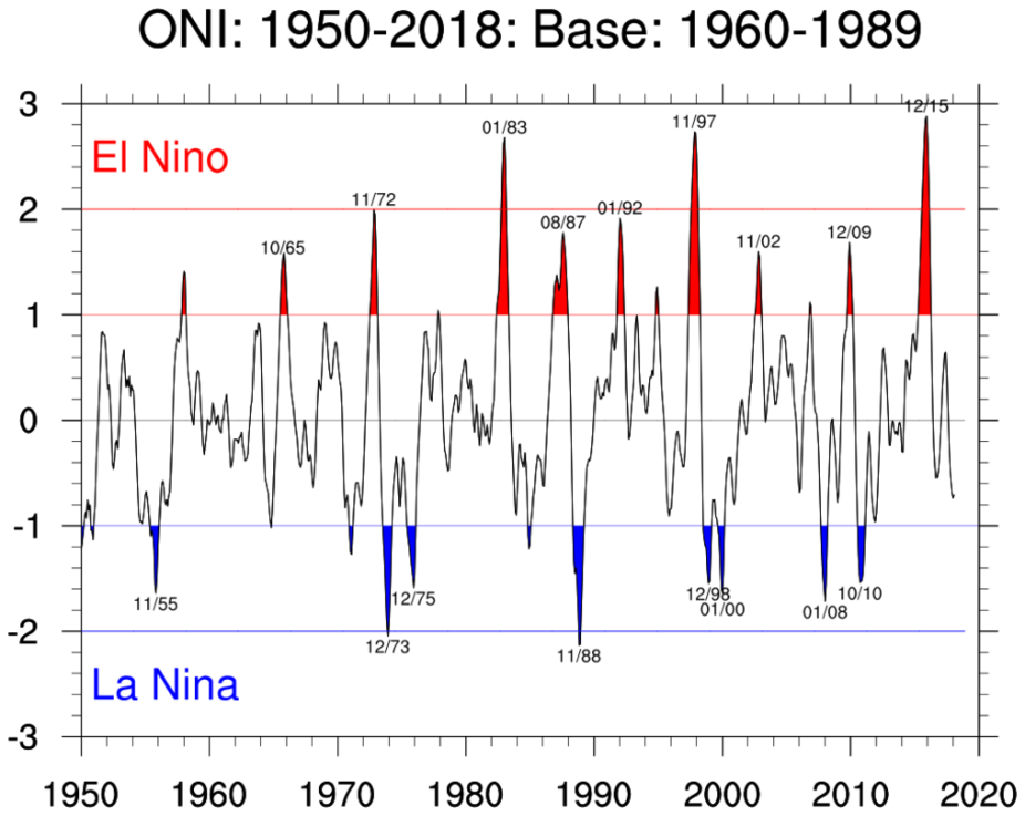
Niño 3.4 (5N-5S, 170W-120W): The Niño 3.4 anomalies may be thought of as representing the average equatorial SSTs across the Pacific from about the dateline to the South American coast. The Niño 3.4 index typically uses a 5-month running mean, and El Niño or La Niña events are defined when the Niño 3.4 SSTs exceed +/- 0.4C for a period of six months or more.
Nino X Index computation: (a) Compute area averaged total SST from Niño X region; (b) Compute monthly climatology (e.g., 1950-1979) for area averaged total SST from Niño X region, and subtract climatology from area averaged total SST time series to obtain anomalies; © Smooth the anomalies with a 5-month running mean; (d) Normalize the smoothed values by its standard deviation over the climatological period.
At the end of this notebook, you should be able to produce a plot that looks similar to this Oceanic Niño Index plot:
Open the SST and areacello datasets, and use Xarray’s merge method to combine them into a single dataset:
filepath = DATASETS.fetch('CESM2_sst_data.nc')
data = xr.open_dataset(filepath)
filepath2 = DATASETS.fetch('CESM2_grid_variables.nc')
areacello = xr.open_dataset(filepath2).areacello

ds = xr.merge([data, areacello])
ds
Downloading file 'CESM2_sst_data.nc' from 'https://github.com/ProjectPythia/pythia-datasets/raw/main/data/CESM2_sst_data.nc' to '/home/runner/.cache/pythia-datasets'.
/usr/share/miniconda/envs/pythia-book-dev/lib/python3.8/site-packages/xarray/conventions.py:523: SerializationWarning: variable 'tos' has multiple fill values {1e+20, 1e+20}, decoding all values to NaN.
  new_vars[k] = decode_cf_variable(
Downloading file 'CESM2_grid_variables.nc' from 'https://github.com/ProjectPythia/pythia-datasets/raw/main/data/CESM2_grid_variables.nc' to '/home/runner/.cache/pythia-datasets'.
<xarray.Dataset>
Dimensions:    (time: 180, d2: 2, lat: 180, lon: 360)
Coordinates:
  * time       (time) object 2000-01-15 12:00:00 ... 2014-12-15 12:00:00
  * lat        (lat) float64 -89.5 -88.5 -87.5 -86.5 ... 86.5 87.5 88.5 89.5
  * lon        (lon) float64 0.5 1.5 2.5 3.5 4.5 ... 356.5 357.5 358.5 359.5
Dimensions without coordinates: d2
Data variables:
    time_bnds  (time, d2) object ...
    lat_bnds   (lat, d2) float64 ...
    lon_bnds   (lon, d2) float64 ...
    tos        (time, lat, lon) float32 ...
    areacello  (lat, lon) float64 ...
Attributes: (12/45)
    Conventions:            CF-1.7 CMIP-6.2
    activity_id:            CMIP
    branch_method:          standard
    branch_time_in_child:   674885.0
    branch_time_in_parent:  219000.0
    case_id:                972
    ...                     ...
    sub_experiment_id:      none
    table_id:               Omon
    tracking_id:            hdl:21.14100/2975ffd3-1d7b-47e3-961a-33f212ea4eb2
    variable_id:            tos
    variant_info:           CMIP6 20th century experiments (1850-2014) with C...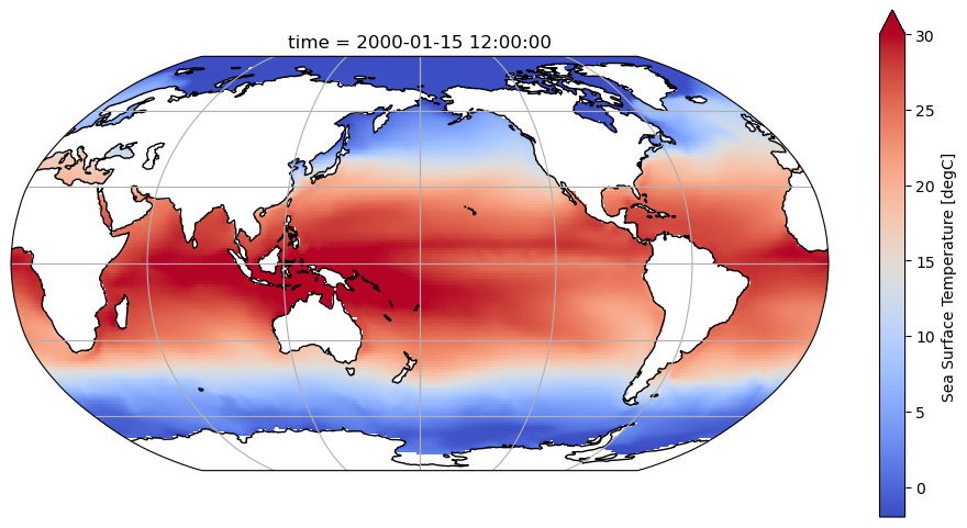
variant_label: r11i1p1f1Visualize the first time slice to make sure the data looks as expected:
fig = plt.figure(figsize=(12, 6))
ax = plt.axes(projection=ccrs.Robinson(central_longitude=180))
ax.coastlines()
ax.gridlines()
ds.tos.isel(time=0).plot(
    ax=ax, transform=ccrs.PlateCarree(), vmin=-2, vmax=30, cmap='coolwarm'
);
/usr/share/miniconda/envs/pythia-book-dev/lib/python3.8/site-packages/cartopy/io/__init__.py:241: DownloadWarning: Downloading: https://naturalearth.s3.amazonaws.com/110m_physical/ne_110m_coastline.zip
  warnings.warn(f'Downloading: {url}', DownloadWarning)
Select the Niño 3.4 region
There are a couple ways to select the Niño 3.4 region:
Use
sel()orisel()Use
where()and select all values within the bounds of interest
tos_nino34 = ds.sel(lat=slice(-5, 5), lon=slice(190, 240))
tos_nino34
<xarray.Dataset>
Dimensions:    (time: 180, d2: 2, lat: 10, lon: 50)
Coordinates:
  * time       (time) object 2000-01-15 12:00:00 ... 2014-12-15 12:00:00
  * lat        (lat) float64 -4.5 -3.5 -2.5 -1.5 -0.5 0.5 1.5 2.5 3.5 4.5
  * lon        (lon) float64 190.5 191.5 192.5 193.5 ... 236.5 237.5 238.5 239.5
Dimensions without coordinates: d2
Data variables:
    time_bnds  (time, d2) object ...
    lat_bnds   (lat, d2) float64 ...
    lon_bnds   (lon, d2) float64 ...
    tos        (time, lat, lon) float32 ...
    areacello  (lat, lon) float64 ...
Attributes: (12/45)
    Conventions:            CF-1.7 CMIP-6.2
    activity_id:            CMIP
    branch_method:          standard
    branch_time_in_child:   674885.0
    branch_time_in_parent:  219000.0
    case_id:                972
    ...                     ...
    sub_experiment_id:      none
    table_id:               Omon
    tracking_id:            hdl:21.14100/2975ffd3-1d7b-47e3-961a-33f212ea4eb2
    variable_id:            tos
    variant_info:           CMIP6 20th century experiments (1850-2014) with C...
variant_label: r11i1p1f1The other option for selecting our region of interest is to use
tos_nino34 = ds.where(
    (ds.lat < 5) & (ds.lat > -5) & (ds.lon > 190) & (ds.lon < 240), drop=True
)
tos_nino34
<xarray.Dataset>
Dimensions:    (time: 180, d2: 2, lat: 10, lon: 50)
Coordinates:
  * time       (time) object 2000-01-15 12:00:00 ... 2014-12-15 12:00:00
  * lat        (lat) float64 -4.5 -3.5 -2.5 -1.5 -0.5 0.5 1.5 2.5 3.5 4.5
  * lon        (lon) float64 190.5 191.5 192.5 193.5 ... 236.5 237.5 238.5 239.5
Dimensions without coordinates: d2
Data variables:
    time_bnds  (time, d2, lat, lon) object 2000-01-01 00:00:00 ... 2015-01-01...
    lat_bnds   (lat, d2, lon) float64 -5.0 -5.0 -5.0 -5.0 ... 5.0 5.0 5.0 5.0
    lon_bnds   (lon, d2, lat) float64 190.0 190.0 190.0 ... 240.0 240.0 240.0
    tos        (time, lat, lon) float32 28.26 28.16 28.06 ... 28.54 28.57 28.63
    areacello  (lat, lon) float64 1.233e+10 1.233e+10 ... 1.233e+10 1.233e+10
Attributes: (12/45)
    Conventions:            CF-1.7 CMIP-6.2
    activity_id:            CMIP
    branch_method:          standard
    branch_time_in_child:   674885.0
    branch_time_in_parent:  219000.0
    case_id:                972
    ...                     ...
    sub_experiment_id:      none
    table_id:               Omon
    tracking_id:            hdl:21.14100/2975ffd3-1d7b-47e3-961a-33f212ea4eb2
    variable_id:            tos
    variant_info:           CMIP6 20th century experiments (1850-2014) with C...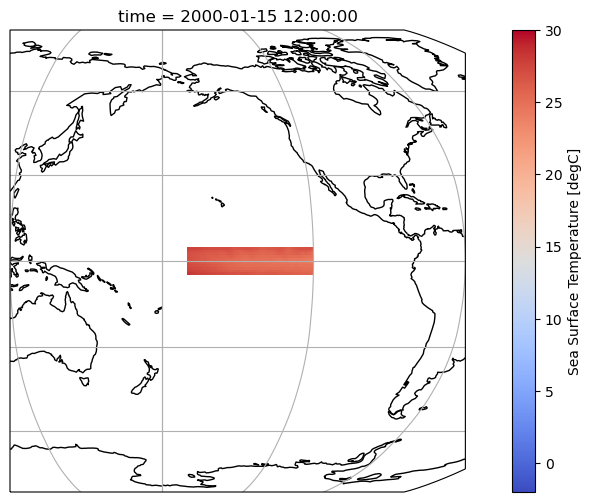
variant_label: r11i1p1f1Let’s plot the selected region to make sure we are doing the right thing.
fig = plt.figure(figsize=(12, 6))
ax = plt.axes(projection=ccrs.Robinson(central_longitude=180))
ax.coastlines()
ax.gridlines()
tos_nino34.tos.isel(time=0).plot(
    ax=ax, transform=ccrs.PlateCarree(), vmin=-2, vmax=30, cmap='coolwarm'
)
ax.set_extent((120, 300, 10, -10))
Compute the anomalies
We first group by month and subtract the mean SST at each point in the Niño 3.4 region. We then compute the weighted average over the region to obtain the anomalies:
gb = tos_nino34.tos.groupby('time.month')
tos_nino34_anom = gb - gb.mean(dim='time')
index_nino34 = tos_nino34_anom.weighted(tos_nino34.areacello).mean(dim=['lat', 'lon'])
Now, smooth the anomalies with a 5-month running mean:
index_nino34_rolling_mean = index_nino34.rolling(time=5, center=True).mean()
index_nino34.plot(size=8)
index_nino34_rolling_mean.plot()
plt.legend(['anomaly', '5-month running mean anomaly'])
plt.title('SST anomaly over the Niño 3.4 region');
---------------------------------------------------------------------------
TypeError                                 Traceback (most recent call last)
Cell In [9], line 1
----> 1 index_nino34.plot(size=8)
      2 index_nino34_rolling_mean.plot()
      3 plt.legend(['anomaly', '5-month running mean anomaly'])

File /usr/share/miniconda/envs/pythia-book-dev/lib/python3.8/site-packages/xarray/plot/accessor.py:46, in DataArrayPlotAccessor.__call__(self, **kwargs)
     44 @functools.wraps(dataarray_plot.plot, assigned=("__doc__", "__annotations__"))
     45 def __call__(self, **kwargs) -> Any:
---> 46     return dataarray_plot.plot(self._da, **kwargs)

File /usr/share/miniconda/envs/pythia-book-dev/lib/python3.8/site-packages/xarray/plot/dataarray_plot.py:312, in plot(darray, row, col, col_wrap, ax, hue, subplot_kws, **kwargs)
    308     plotfunc = hist
    310 kwargs["ax"] = ax
--> 312 return plotfunc(darray, **kwargs)

File /usr/share/miniconda/envs/pythia-book-dev/lib/python3.8/site-packages/xarray/plot/dataarray_plot.py:517, in line(darray, row, col, figsize, aspect, size, ax, hue, x, y, xincrease, yincrease, xscale, yscale, xticks, yticks, xlim, ylim, add_legend, _labels, *args, **kwargs)
    513 ylabel = label_from_attrs(yplt, extra=y_suffix)
    515 _ensure_plottable(xplt_val, yplt_val)
--> 517 primitive = ax.plot(xplt_val, yplt_val, *args, **kwargs)
    519 if _labels:
    520     if xlabel is not None:

File /usr/share/miniconda/envs/pythia-book-dev/lib/python3.8/site-packages/matplotlib/axes/_axes.py:1664, in Axes.plot(self, scalex, scaley, data, *args, **kwargs)
   1662 lines = [*self._get_lines(*args, data=data, **kwargs)]
   1663 for line in lines:
-> 1664     self.add_line(line)
   1665 if scalex:
   1666     self._request_autoscale_view("x")

File /usr/share/miniconda/envs/pythia-book-dev/lib/python3.8/site-packages/matplotlib/axes/_base.py:2340, in _AxesBase.add_line(self, line)
   2337 if line.get_clip_path() is None:
   2338     line.set_clip_path(self.patch)
-> 2340 self._update_line_limits(line)
   2341 if not line.get_label():
   2342     line.set_label(f'_child{len(self._children)}')

File /usr/share/miniconda/envs/pythia-book-dev/lib/python3.8/site-packages/matplotlib/axes/_base.py:2363, in _AxesBase._update_line_limits(self, line)
   2359 def _update_line_limits(self, line):
   2360     """
   2361     Figures out the data limit of the given line, updating self.dataLim.
   2362     """
-> 2363     path = line.get_path()
   2364     if path.vertices.size == 0:
   2365         return

File /usr/share/miniconda/envs/pythia-book-dev/lib/python3.8/site-packages/matplotlib/lines.py:1031, in Line2D.get_path(self)
   1029 """Return the `~matplotlib.path.Path` associated with this line."""
   1030 if self._invalidy or self._invalidx:
-> 1031     self.recache()
   1032 return self._path

File /usr/share/miniconda/envs/pythia-book-dev/lib/python3.8/site-packages/matplotlib/lines.py:659, in Line2D.recache(self, always)
    657 if always or self._invalidx:
    658     xconv = self.convert_xunits(self._xorig)
--> 659     x = _to_unmasked_float_array(xconv).ravel()
    660 else:
    661     x = self._x

File /usr/share/miniconda/envs/pythia-book-dev/lib/python3.8/site-packages/matplotlib/cbook/__init__.py:1369, in _to_unmasked_float_array(x)
   1367     return np.ma.asarray(x, float).filled(np.nan)
   1368 else:
-> 1369     return np.asarray(x, float)

TypeError: float() argument must be a string or a number, not 'cftime._cftime.DatetimeNoLeap'
Compute the standard deviation of the SST in the Nino 3.4 region, over the entire time period of the data array:
std_dev = tos_nino34.tos.std()
std_dev
<xarray.DataArray 'tos' ()>
array(1.8436452, dtype=float32)
Then we’ll normalize the values by dividing the rolling mean by the standard deviation of the SST in the Niño 3.4 region:
normalized_index_nino34_rolling_mean = index_nino34_rolling_mean / std_dev
Visualize the computed Niño 3.4 index
We will highlight values in excess of \(\pm\)0.5, roughly corresponding to El Niño (warm) and La Niña (cold) events.
fig = plt.figure(figsize=(12, 6))

plt.fill_between(
    normalized_index_nino34_rolling_mean.time.data,
    normalized_index_nino34_rolling_mean.where(
        normalized_index_nino34_rolling_mean >= 0.4
    ).data,
    0.4,
    color='red',
    alpha=0.9,
)
plt.fill_between(
    normalized_index_nino34_rolling_mean.time.data,
    normalized_index_nino34_rolling_mean.where(
        normalized_index_nino34_rolling_mean <= -0.4
    ).data,
    -0.4,
    color='blue',
    alpha=0.9,
)

normalized_index_nino34_rolling_mean.plot(color='black')
plt.axhline(0, color='black', lw=0.5)
plt.axhline(0.4, color='black', linewidth=0.5, linestyle='dotted')
plt.axhline(-0.4, color='black', linewidth=0.5, linestyle='dotted')
plt.title('Niño 3.4 Index');
---------------------------------------------------------------------------
TypeError                                 Traceback (most recent call last)
Cell In [12], line 3
      1 fig = plt.figure(figsize=(12, 6))
----> 3 plt.fill_between(
      4     normalized_index_nino34_rolling_mean.time.data,
      5     normalized_index_nino34_rolling_mean.where(
      6         normalized_index_nino34_rolling_mean >= 0.4
      7     ).data,
      8     0.4,
      9     color='red',
     10     alpha=0.9,
     11 )
     12 plt.fill_between(
     13     normalized_index_nino34_rolling_mean.time.data,
     14     normalized_index_nino34_rolling_mean.where(
   (...)
     19     alpha=0.9,
     20 )
     22 normalized_index_nino34_rolling_mean.plot(color='black')

File /usr/share/miniconda/envs/pythia-book-dev/lib/python3.8/site-packages/matplotlib/pyplot.py:2526, in fill_between(x, y1, y2, where, interpolate, step, data, **kwargs)
   2522 @_copy_docstring_and_deprecators(Axes.fill_between)
   2523 def fill_between(
   2524         x, y1, y2=0, where=None, interpolate=False, step=None, *,
   2525         data=None, **kwargs):
-> 2526     return gca().fill_between(
   2527         x, y1, y2=y2, where=where, interpolate=interpolate, step=step,
   2528         **({"data": data} if data is not None else {}), **kwargs)

File /usr/share/miniconda/envs/pythia-book-dev/lib/python3.8/site-packages/matplotlib/__init__.py:1423, in _preprocess_data.<locals>.inner(ax, data, *args, **kwargs)
   1420 @functools.wraps(func)
   1421 def inner(ax, *args, data=None, **kwargs):
   1422     if data is None:
-> 1423         return func(ax, *map(sanitize_sequence, args), **kwargs)
   1425     bound = new_sig.bind(ax, *args, **kwargs)
   1426     auto_label = (bound.arguments.get(label_namer)
   1427                   or bound.kwargs.get(label_namer))

File /usr/share/miniconda/envs/pythia-book-dev/lib/python3.8/site-packages/matplotlib/axes/_axes.py:5367, in Axes.fill_between(self, x, y1, y2, where, interpolate, step, **kwargs)
   5365 def fill_between(self, x, y1, y2=0, where=None, interpolate=False,
   5366                  step=None, **kwargs):
-> 5367     return self._fill_between_x_or_y(
   5368         "x", x, y1, y2,
   5369         where=where, interpolate=interpolate, step=step, **kwargs)

File /usr/share/miniconda/envs/pythia-book-dev/lib/python3.8/site-packages/matplotlib/axes/_axes.py:5272, in Axes._fill_between_x_or_y(self, ind_dir, ind, dep1, dep2, where, interpolate, step, **kwargs)
   5268         kwargs["facecolor"] = \
   5269             self._get_patches_for_fill.get_next_color()
   5271 # Handle united data, such as dates
-> 5272 ind, dep1, dep2 = map(
   5273     ma.masked_invalid, self._process_unit_info(
   5274         [(ind_dir, ind), (dep_dir, dep1), (dep_dir, dep2)], kwargs))
   5276 for name, array in [
   5277         (ind_dir, ind), (f"{dep_dir}1", dep1), (f"{dep_dir}2", dep2)]:
   5278     if array.ndim > 1:

File /usr/share/miniconda/envs/pythia-book-dev/lib/python3.8/site-packages/numpy/ma/core.py:2366, in masked_invalid(a, copy)
   2364     cls = type(a)
   2365 else:
-> 2366     condition = ~(np.isfinite(a))
   2367     cls = MaskedArray
   2368 result = a.view(cls)

TypeError: ufunc 'isfinite' not supported for the input types, and the inputs could not be safely coerced to any supported types according to the casting rule ''safe''
Summary
We have applied a variety of Xarray’s selection, grouping, and statistical functions to compute and visualize an important climate index.
Resources and References
Matplotlib’s
axhlinemethod (see also its analogousaxvlinemethod)